Manual
Theoretical and technical details of RD NMR are discussed in this document
Goals: Background on CPMG RD method, Details on GUARDD data organization, features, and reference materials
Scientific questions addressed by RD NMR
- Question: Is this molecule flexible in the μs-ms time window?
- If the Rex of an RD NMR experiment > 0, it will be flexible on this timescale
- Question: If so, what is the nature of this exchange process?
- Typically, exchange processes are considered as at least one site of a single molecule which occupies at least two distinct local structures (AKA states or configurations), denoted A and B
- Question: What is the chemical environment (e.g., structure) of
this alternate configuration?
- The chemical shift difference Δω obtained from at least one RD NMR experiment informs on this question
- Question: On average, how often is this alternate configuration
sampled?
- Answer: The total exchange rate kex from at least one RD NMR experiment indicates the rate of interconversion between the A and B states
- Question: What is the relative population of this alternate
configuration?
- Answer: via population PA from at least one RD NMR experiment
- Question: How much activation energy is required to access this
alternate configuration?
- Answer: via activation energies E(A→B) and E(B→A) from several RD experiments (Arrhenius analysis)
- Question: What is the relative energy, enthalpy and entropy of this
alternate configuration?
- Answer: via energy ΔG (via PA), enthalpy ΔH, entropy ΔS from several RD experiments (van’t Hoff analysis)
- Question: Is the alternate configuration a well-defined fold? Is it
unfolded?
- Answer: via chemical shift difference Δω, enthalpy ΔH, entropy ΔS from several RD experiments (See Kleckner & Foster, 2011
- Question: Are motions in this molecule unified, coupled or
independent?
- Answer: via exchange rates kA and kB, enthalpy ΔH, entropy ΔS and activation energies E(A→B) and E(B→A) for several sites from several RD experiments (See Kleckner & Foster, 2011)
Chemical exchange phenomenon
Adapted from Kleckner and Foster, 2011
- Certain dynamic processes in the μs-ms time window lead to characteristic broadening of the NMR signal
- This “exchange broadening” can obscure the observables and in some cases render the NMR signal undetectable
- However, this contains valuable information on the underlying dynamic process
- The relaxation dispersion (RD) NMR experiment can access this information by use of a spin-echo pulse train
The RD experiment refocuses chemical exchange broadening Rex
- Carr-Purcell Meiboom-Gill Relaxation Dispersion (CPMG RD) uses spin-echo pulse trains to suppress relaxation due to exchange processes on the µs-ms timescale.
- (a) The number of spin-echo pulses applied during the fixed
relaxation time directly determines the CPMG frequency via νCPMG = 1 / (4τ).
- The applied CPMG pulse train is shown above each relaxation delay (νCPMG = 100, 500 and 1100 Hz).
- These pulses reduce the signal relaxation rate during the relaxation delay by refocusing exchange broadening (i.e., reducing Rex).
- (b) The observed signal intensity remaining at the end of the TCPMG relaxation delay is used to obtain an effective relaxation rate, where I0 is the signal intensity in the absence of the relaxation delay (i.e., when TCPMG = 0).
- (c) The dispersion Curve reports on dynamics by plotting relaxation rate as a function of refocusing frequency.

Two-state exchange model
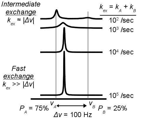
- A single NMR probe (e.g., Ala 12NH) is considered to alternate between local structures designated A and B, which have distinct NMR chemical shifts in 1H and/or AX dimensions.
- Although two signals are shown here, the “minor” B state is not detected directly because its NMR signal is too weak and/or too broad.
- However, the A↔B exchange yields a quantitative effect on the measured RD Curve of signal A.

The two-state exchange model requires 4-5 parameters to describe a single RD Curve
Structural parameters (1 or 2 per NMR probe)
- |(ΔωH)| (rad/s): Magnitude of 1H chemical shift difference between A and B states (for MQ Curves only)
- |(ΔωX)| (rad/s): Magnitude of AX chemical shift difference between A and B states (AX = 13C or 15N)
Kinetic parameters (2 per temperature per NMR probe)
Parameters used in fitting equations
- kex (/s): Total exchange rate between state A and B; kex = kA + kB
- PA (-): Population fraction of state A; PA = kB / (kA + kB) with PA + PB = 1 * Alternate physical parameterization, which requires knowledge of both kex and PA
- kA (/s): Average frequency (not velocity!) of transition from state A to state B
- kB (/s): Average frequency (not velocity!) of transition from state B to state A
Relaxation parameter (1 per Curve per NMR probe)
- R20 (Hz): Relaxation rate of the A state in the absence of exchange
- The MQ Curve shown here is simulated using |ΔωH| = 8 Hz, Abs(ΔωX) = 201 Hz, kex = 1000 /s, PA = 90%,and = 10 Hz.
Assigning parameters for fitting
Fitting requries five parameters per Curve, but often parameters can be shared when Curves are aggregated into Curvesets, which are aggregated into Groups
Details on Curves, Curvesets, and Groups can be found later in the Manual s .. image:: figures/figure-data_management-example.png
Figure above (a) Hierarchical data structures used in GUARDD, (b) example data structure
- Each Curve is designated a unique R20
- R20 = Transverse relaxation rate in the absence of exchange (Hz)
- Assume: Relaxation rates of states A and B are equal (R2A0 = R2B0)
- One or more Curves are aggregated into a Curveset, which designate
the same chemical shift differences |ΔωH| and |ΔωX|
- Assume: |ΔωH| (ppm) and |ΔωX| (ppm) are independent
of temperature
- Therefore, each unique temperature yields an independent measure of |ΔωH| and/or |ΔωX|
- NMR: Resonance frequency scales with magnetic field strength
- Therefore, each unique B0 field yields an independent measure of |ΔωX|
- See calculations for converting between rad/s and ppm later in the Manual
- NMR: An experiment may be designed to detect a particular
quantum coherence
- Therefore, each unique quantum coherence yields an independent measure of |ΔωH| and/or |ΔωX|
- Single Quantum (SQ) experiments are sensitive to only |ΔωH| or |ΔωX|
- Multiple Quantum (MQ) experiments are sensitive to the sum |ΔωH + ΔωX|
- See Korzhnev, et al. (2005)
- More information on Quantum Coherences in dispersion are covered later.
- Assume: |ΔωH| (ppm) and |ΔωX| (ppm) are independent
of temperature
- One or more Curvesets are aggregated into a Group, which designates
the kinetic parameters (PA and kex at each temperature)
- Physics: Kinetic parameters are determined by experimental
conditions
- E.g., temperature, buffer, sometimes concentration but NOT magnetic field strength
- Therefore, each repeat condition (same or different B0) yields an independent measure of PA and kex
- There are at least two methods to specify PA and kex at each temperature
- Method A - No constraint on rate analysis
- Define PA and kex at each temperature explicitly
- Method B - Constrain rate analysis via ΔH and EAB
- Define PA and kex at a single temperature, T0
- Define ΔH for temperature-dependence of PA (vant Hoff)
- Define EAB for temperature-dependence of kA and, using ΔH, kB and therefore kex = kA +kB (Arrhenius)
- See calculations in the Arrhenius section of this Manual
- Physics: Kinetic parameters are determined by experimental
conditions
Example parameter assignment
Check the command window output for itemization of each parameter in a given Group
Usethe debugging output option
OUTPUT_DEBUG_UPDATE_FIT_PARAMS
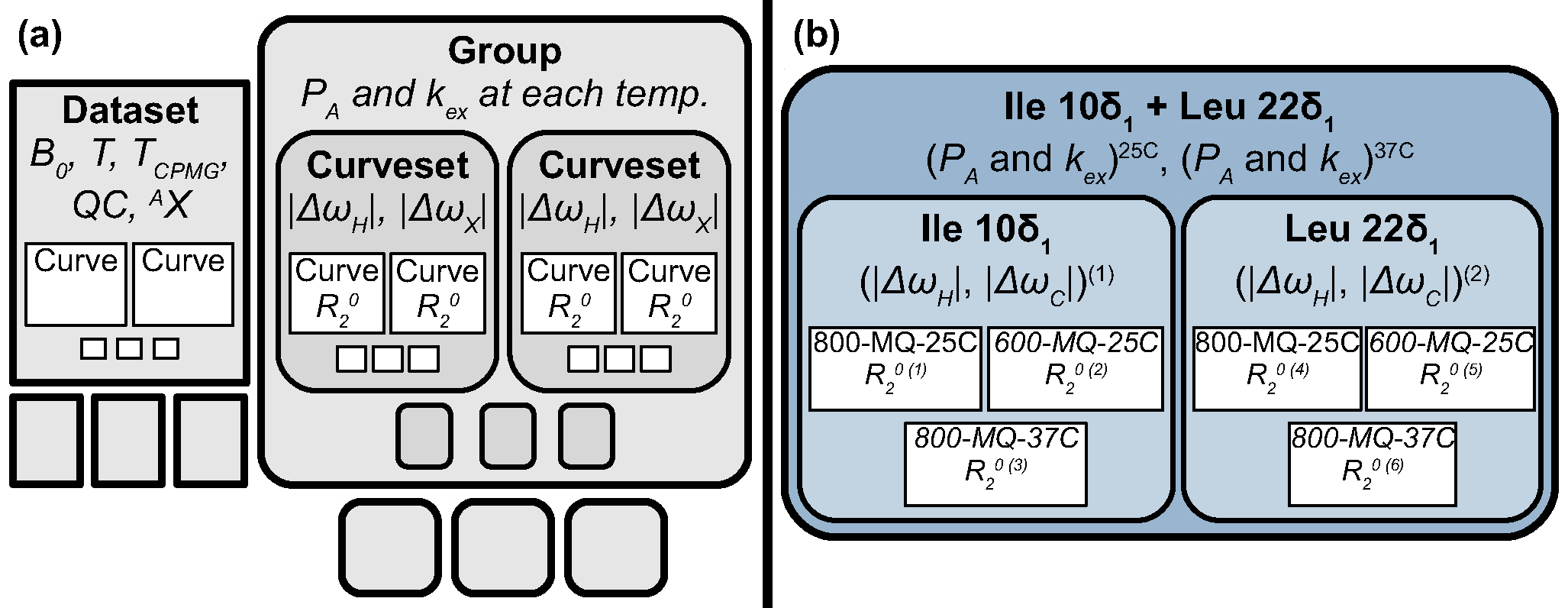
Figure above (a) Hierarchical data structures used in GUARDD, (b) example data structure discussed below*
- Goal: Show two ways (A or B) to itemize temperature-depenence of PA and kex
- Example: Method A - No constraint on rate analysis
- Define PA and kex at each temperature
- Notation
- CS = Curveset number (1 or 2)
- C = Curve number within the Curveset (1, 2, or 3)
- CTOT = Total Curve number within the Group (1, 2, 3, 4, 5, or 6)
FUNCTION: Group.updateFitParams
    Working on CS=1, Ile 10\delta_1
    Working on C=1 (CTOT=1), 800-MQ-25C
            Itemizing parameter 1 (dwH @ CS1, C1)
            Itemizing parameter 2 (dwX @ CS1, C1)
            Itemizing parameter 3 (PA @ 298K) *PA0*
            Itemizing parameter 4 (kex @ 298K) *kex0*
            Itemizing parameter 5 (R20 @ CS1, C1)
    Working on C=2 (CTOT=2), 600-MQ-25C
            Linking dwH to parameter 1, scaled by 0.750091x
            Linking dwX to parameter 2, scaled by 0.750091x
            Linking PA to parameter 3, scaled by 1.000000x
            Linking kex to parameter 4, scaled by 1.000000x
            Itemizing parameter 6 (R20 @ CS1, C2)
    Working on C=3 (CTOT=3), 800-MQ-37C
            Linking dwH to parameter 1, scaled by 1.000000x
            Linking dwX to parameter 2, scaled by 1.000000x
            Itemizing parameter 7 (PA @ 310K) *PA0*
            Itemizing parameter 8 (kex @ 310K) *kex0*
            Itemizing parameter 9 (R20 @ CS1, C3)
    Working on CS=2, Leu 22\delta_1
    Working on C=1 (CTOT=4), 800-MQ-25C
            Itemizing parameter 10 (dwH @ CS2, C1)
            Itemizing parameter 11 (dwX @ CS2, C1)
            Linking PA to parameter 3, scaled by 1.000000x
            Linking kex to parameter 4, scaled by 1.000000x
            Itemizing parameter 12 (R20 @ CS2, C1)
    Working on C=2 (CTOT=5), 600-MQ-25C
            Linking dwH to parameter 10, scaled by 0.750091x
            Linking dwX to parameter 11, scaled by 0.750091x
            Linking PA to parameter 3, scaled by 1.000000x
            Linking kex to parameter 4, scaled by 1.000000x
            Itemizing parameter 13 (R20 @ CS2, C2)
    Working on C=3 (CTOT=6), 800-MQ-37C
            Linking dwH to parameter 10, scaled by 1.000000x
            Linking dwX to parameter 11, scaled by 1.000000x
            Linking PA to parameter 7, scaled by 1.000000x
            Linking kex to parameter 8, scaled by 1.000000x
            Itemizing parameter 14 (R20 @ CS2, C3)
- *Example: Method B - Constrain rate analysis via ΔH and EAB*
- Define PA and kex at a single temperature, T0
- Define ΔH for temperature-dependence of PA (vant Hoff)
- Define EAB for temperature-dependence of kA and, using ΔH, kB and therefore kex = kA +kB (Arrhenius)
- Note: this uses ΔH and EAB instead of PA(37C) and kex(37C)
FUNCTION: Group.updateFitParams
             Number of temperatures 2 > 1
             Itemizing parameter 1 (dH)
             Itemizing parameter 2 (Eab)
     Working on CS=1, Ile 10\delta_1
     Working on C=1 (CTOT=1), 800-MQ-25C
             Itemizing parameter 3 (dwH @ CS1, C1)
             Itemizing parameter 4 (dwX @ CS1, C1)
             Itemizing parameter 5 (PA @ 298K) *PA0*
             Itemizing parameter 6 (kex @ 298K) *kex0*
             Itemizing parameter 7 (R20 @ CS1, C1)
     Working on C=2 (CTOT=2), 600-MQ-25C
             Linking dwH to parameter 3, scaled by 0.750091x
             Linking dwX to parameter 4, scaled by 0.750091x
             Linking PA to parameter 5, scaled by 1.000000x
             Linking kex to parameter 6, scaled by 1.000000x
             Itemizing parameter 8 (R20 @ CS1, C2)
     Working on C=3 (CTOT=3), 800-MQ-37C
             Linking dwH to parameter 3, scaled by 1.000000x
             Linking dwX to parameter 4, scaled by 1.000000x
             Linking PA @ 310K to PA0 @ T0=298K (param 5) via Temp (310K), dH (param 1), and Eab (param 2)
             Linking kex @ 310K to kex0 @ T0=298K (param 6) via Temp (310K), dH (param 1), and Eab (param 2)
             Itemizing parameter 9 (R20 @ CS1, C3)
     Working on CS=2, Leu 22\delta_1
     Working on C=1 (CTOT=4), 800-MQ-25C
             Itemizing parameter 10 (dwH @ CS2, C1)
             Itemizing parameter 11 (dwX @ CS2, C1)
             Linking PA to parameter 5, scaled by 1.000000x
             Linking kex to parameter 6, scaled by 1.000000x
             Itemizing parameter 12 (R20 @ CS2, C1)
     Working on C=2 (CTOT=5), 600-MQ-25C
             Linking dwH to parameter 10, scaled by 0.750091x
             Linking dwX to parameter 11, scaled by 0.750091x
             Linking PA to parameter 5, scaled by 1.000000x
             Linking kex to parameter 6, scaled by 1.000000x
             Itemizing parameter 13 (R20 @ CS2, C2)
     Working on C=3 (CTOT=6), 800-MQ-37C
             Linking dwH to parameter 10, scaled by 1.000000x
             Linking dwX to parameter 11, scaled by 1.000000x
             Linking PA to parameter 5, scaled by 1.000000x
             Linking kex to parameter 6, scaled by 1.000000x
             Itemizing parameter 14 (R20 @ CS2, C3)
Organizing data
Goal: Organize data in hierarchical manner to provide framework for fitting procedures
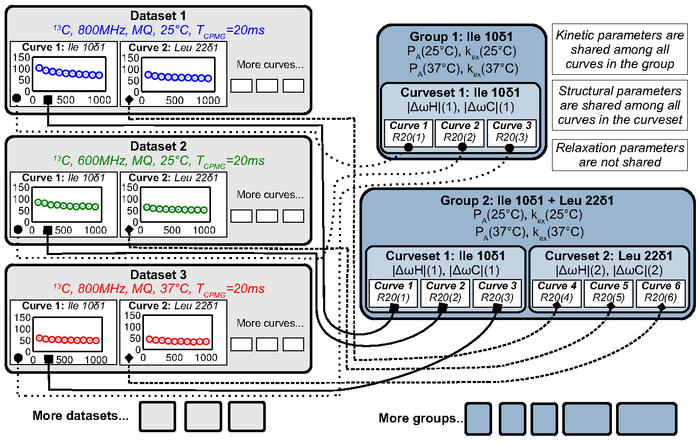
Figure above Datasets contain Curves, which are linked to by Curvesets within Groups
Dataset
Goal: Store a CPMG NMR dataset and the experimental conditions during acquisition
- Properties
- name: Name of dataset (e.g., ‘MQ 800MHz 25C’)
- AX_String: 13C or 15N
- **B0**: Magnetic field strength (1H MHz)
- Temp: Temperature (K)
- TCPMG: Total CPMG time in pulse sequence
- SQX: True=Single Quantum dataset (ΔωH fixed to zero), False=Multiple Quantum dataset (ΔωH may be non-zero)
- Data for each dispersion Curve
- Intensity values and errors
- R2eff values and errors
- νCPMG values
- Pointers to Curves which also hold this information
Key functions in code
Dataset.m
- Add a single RD curve to the dataset
addData
calculateR2eff
calculateErrorsUsingDuplicates
enforceMinimumError
readNlin
Curve
Goal: Store an NMR dispersion Curve (R2Eff (νCPMG)) and the experimental conditions during acquisition, which correspond to its parent.
- Properties
- Properties from its parent Dataset (copied to each
Curve for convenience)
- AX_String: 13C or 15N
- **B0**: Magnetic field strength (1H MHz)
- Temp: Temperature (K)
- TCPMG: Total CPMG time in pulse sequence
- SQX: True=Single Quantum dataset (ΔωH fixed to zero), False=Multiple Quantum dataset (ΔωH may be non-zero)
- Data from its parent Dataset (copied to each Curve
for convenieice)
- Nobs: Number of observations
- vcpmg: Array of vcpmg values (Hz)
- R2eff: Array of R2eff values (Hz)
- eR2eff: Array of errors in R2eff (Hz)
- Each Curve is unique, but can have multiple appearances, each of
which points to the same source data
- Multiple appearances can occur in different Curvesets
- Any changes to a Curve will alter every apperance of that Curve (e.g., in all Curvesets that point to it)
Key functions in code:
Curve.m
- Basic input/output
Curveset
Goal: Store a set of Curves (each from the same NMR probe/assignment) which all share a single pair of chemical shift differences (ΔωH and ΔωX)
- Properties
- name: Name of Curveset
- index: Residue number
- atom: _Name of atom (N, H:raw-latex:alpha, C:raw-latex:delta1, etc.)
- residue: Name of residue (Ile, Leu, Arg, etc.)
- Curvesets contain pointers to Curves (selected from Datasets)
- Nc: Number of Curves in the Curveset
- Pointers to [Manual#Curve Curves] which hold the actual data and experimental conditions
- Each Curveset only appears once (unlike Curves)
Key functions in code:
Curveset.m
- Basic input/output
Group
Goal: Store a Group of Curvesets (each from different NMR probes/assignments) which all share a single set of exchange kinetics (PA and kex at each temperature), and store any Fit Results for this Group
- Properties
- name: Name of Group
- index: Index of the Group (for sorting; this may correspond to residue number)
- Storage of fitting results
- exhibitsExchange: This Group exhibits exchange (true/false)
- bestFitIsOK: The best fit to this Group is OK (true/false)
- Nf: Number of fit results
- fitResults_Grid: Array of FitResults for the grid search
- fitResults: Array of FitResults for arbitrary fits (ex and no-ex)
- fitResult_NoEx: Fit result to no exchange model
- fitResult_Best: Best fit result out of all fits (ex and no-ex)
- Groups contain pointers to Curvesets, each of which only appears once
- Each Group points to a parent Session which contains settings, etc.
Key functions in code:
Group.m
- De-linearize parameter array to matrix form for fitting
delinearizePFmincon
- Return data point (NATURAL UNITS) for the desired parameter, temperature, B0, and Quantum Coherence
getData
- Perform grid search to fit RD data with variety of initial conditions, and return updated fit_results
gridSearch
- Identify the independent parameters and dependent scaling factors for the Group fit
updateFitParams
Fit Result
Goal: Pefrorm a single fit to a Group of RD data, and store the results
- Storage of a single fit result
- Name of fit result
- Use of Arrhenius relation to constrain rate analysis
- Initial conditions for fit parameters
- Final values for fit parameters
- Errors in fit parameters (from Monte Carlo)
- Designation if each parameter is OK or not
- RateAnalysis structure for temperature-dependence
Key functions in code:
FitResult.m
- Analyze the fitResult (usually called after fitMe()
analyzeMe
- Estimate error in dispersion fit using Monte Carlo bootstrapping
calculateErrors
- Fit the Group either to NOEXCHANGE or EXCHANGE model
fitMe
- Set the param_isOK for the parameter name
setParamIsOK
- Simulate the fit (no optimization)
simMe
- Set initial fitting conditions
setInitial_Kinetics_UnconstrainedRates
- Set initial fitting conditions
setInitial_Kinetics_ConstrainedRates
- Set initial fitting conditions for ΔωH, ΔωX, and R20
setInitial_Shifts
Rate Analysis
Goal: Store the results of a temperature-dependent analysis of the PA and kex
- Storage of temperature-dependent parameters
- All Arrhenius parameters
- arrhenius_isOK
- All vant Hoff parameters
- vantHoff_isOK
Key functions in code:
RateAnalyis.m
- Update kinetic quantities using PA(T) and kex(T)
analyzeMe
- Return X and Y vectors for the Arrhenius plots A (ln(kA) vs. 1/T (or ln(kB) vs 1/T))
getArrheniusPlotA
- Return X and Y vectors for van’t Hoff plot (ln(K) vs 1/T)
getVantHoffPlot
Session
Goal: Store the program data and settings
- Store all Datasets
- Store all Groups
Key functions in code:
FitResult.m
- Generate minimal set of NEW Groups to partition Curves via NMR probe (index/atom)
generateGroups
- Generate minimal set of NEW Curvesets to partition Curves via NMR probe (index/atom)
generateCurvesetsForGroup
- Return plot title and axis label for a given parameter name
getPlotLabels
- Return plot symbol character (‘o’, ‘s’, etc.) and colorRGB vector
getPlotSymbolAndColor
- Load 1+ datasets using script file
loadDatasets
- Sort the Groups by index and name
sortGroups
- Convert the parameter units for arbitrary parameter for natural or display units
convertUnits
- Does the parameter need a particular Temp and/or B0?
getParamRequirements
General Use
Acquire and prepare data
Acquire CPMG RD NMR spectra
- Multiple temperatures, B0 fields, SQ and/or MQ dispersion for either 13C or 15N sites
- Extract peak intensities with NMRPipe.
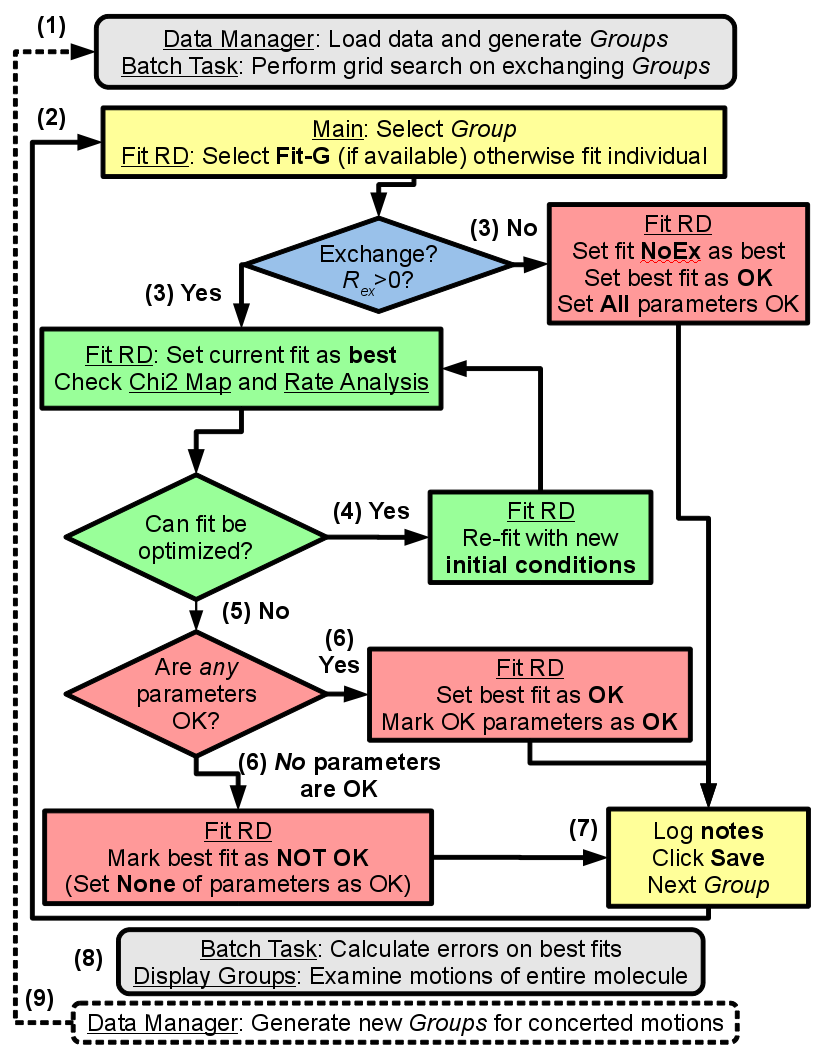
Analyze data using GUARDD
- Load the data and execute the grid search on exchanging Groups
- For each Group, the grid search fit is selected, otherwise an individual fit is performed
- In YES to exchange, the current best fit is evaluated via χ2 maps and rate analyses
- If NO exchange, the NoEx fit is marked for subsequent analysis
- If fitted values can be optimized, the user supplies new initial conditions and re-evaluates the fit at (3)
- If fitted values cannot be optimized, the user designates which ones are valid/invalid, if any
- It is important that invalid parameters be designated as such, lest they be analyzed/displayed in subsequent output
- The user should enter text to describe the fitting result
- Especially if there is work to do (e.g., new Grid Search, multi-Curveset fitting, remove noisy data)
- Once fits are optimized, errors are calculated using Monte Carlo bootstrapping and results are viewed
- New Groups can be generated to test global motions and/or to refine fit results
GUARDD Graphical Interface
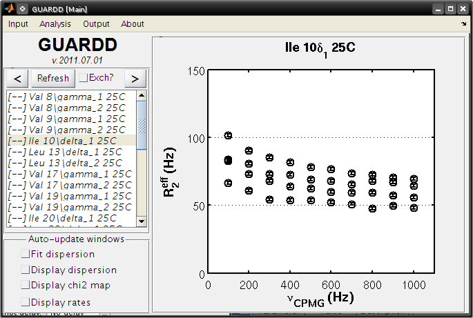
GUARDD Input menu
Clear session
Clears the session, as if the program was just opened
Load session
- Clears the current session
- Loads a previously saved GUARDD session (a “.mat” MATLAB variables file)
- This may take a relatively long time to load
- 1 Mb file takes ~0.5 min
- 10 Mb file takes ~5 min
Settings
Goal: Change program settings here
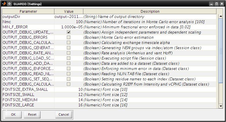
- Take special note of OUTPUT_DEBUG flags, which are helpful to see program logic during execution
- The items on this list are set in the code via {{{Session.param_info}}}
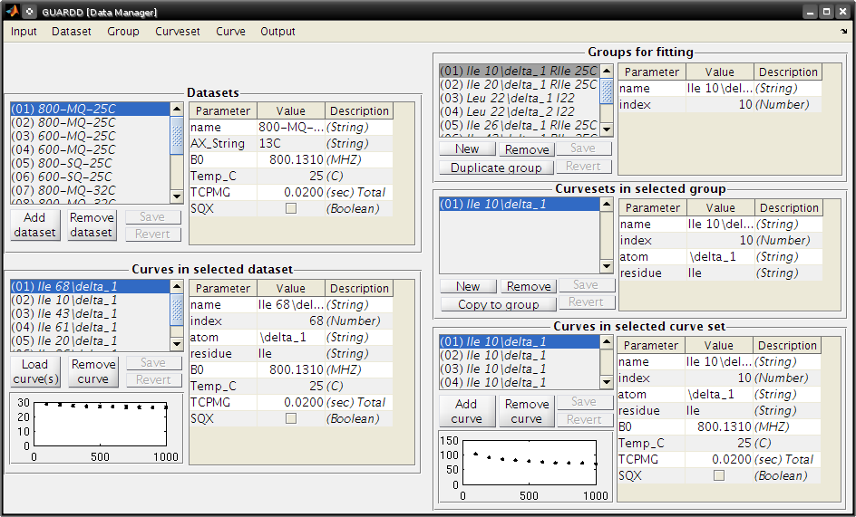
Data Manger
Goal: Manage datasets, Curves, Curvesets, and Groups for analysis (input and basic output)
Menu items
- Input…
- Script…
- Loads a script file
Sequence file…
- Load a sequence file
Dataset…
- Sort Curves (this dataset) → Curves sorted by {{{index}}} and {{{atom}}} are easier to browse
- Sort Curves (all datasets)
Group…
Sort Groups → Groups sorted by index and name are easier to browse
- Code:
Session.sortGroups()
Generate from all data → Generate minimal set of NEW Groups to partition Curves via NMR probe (index and atom)
- Each new Group contains one new Curveset containing all the Curves for that NMR probe
- Code:
Session.generateGroups()
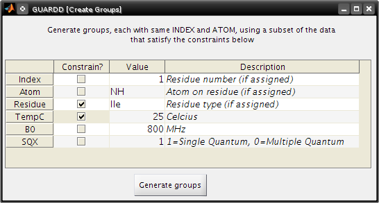
Generate from subsets of data → Same as above, except using Curves from only part of the dataset
- This launches the Create Groups dialog
- Code:
Session.generateGroups()
Curveset…
- Sort Curvesets (this Group)… → Curvesets sorted by index and name are easier to browse
- Generate from alldata… → For the selected Group, generate minimal set of NEW Curvesetsto partition Curves via NMR probe (index and atom)
- This is the easiest way to generate a large Group (e.g., all Curves reporting same dynamic process)
- From here, certain Curvesets and Curves can be removed, if desired
- Copy to Group… → Copy the selected Curveset to another Group
- This launches the Select Group dialog
Curve…
- (Nothing yet)
Output…
Datasets…
- Writes a Dataset file
- Groups…
- Writes a Groups file
Panels and buttons
- Each table contains editable information on the object
- Button: Save → Save changes made to the table
- Button: Revert → Discard changes made to the table
- Panel: Datasets
- Displays all the loaded datasets
- Button: Add dataset → Adds an empty Dataset to the list
- This can be edited and Curves can be loaded manually using nlin.tab file
- This is NOT the preferred method to load data
- Button: Remove dataset → Removes the selected dataset from the list
- Panel: Curves in selected dataset
- Lists all the Curves and displays their properties
- Note: Changing Curve properties here will propagate to all apperances of that Curve
- Button: Load Curve(s) → This is NOT the preferred method to load data
- Button: Remove Curve → Removes the selected Curve from the Dataset (and ALL appearances of that Curve)
- Panel: Groups for fitting
- Lists all the Groups in the Session
- Button: New → Add an empty Group
- Useful for creating custom Groups with desired Curvesets and Curves
- Button: Remove → Remove the selected Group
- Duplicate Group → Copy the Group and all Curvesets within
- Useful for creating custom Groups (e.g., copy then add/remove Curvesets)
- Panel: Curvesets in selected Group
- Displays all the Curvesets in the selected Group
- Button: New → Add an empty Curveset to the selected Group
- Button: Remove → Remove the selected Curveset from the selected Group
- Button: Copy to Group → Copy the selected Curveset to another Group
- This launches the Select Group dialog
- Panel: Curves in selected Curveset
- Displays all the Curves which are pointed to by the selected Curveset
- Note: Changing Curve properties here will propagate to all apperances of that Curve
- Button: Add Curve → Add the Curve that is selected from the Dataset (on the left)
- Button: Remove Curve → Remove the appearance of this Curve from the Curveset (does NOT delete Curve from the dataset)
Create Groups
Goal: Create a set of Groups using a subset of the data
Helpful when only part of a large dataset is desired
- Tutorial: Advanced Group creation
Select Group
Goal: Select a Group so that the selected Curveset can be copied to it
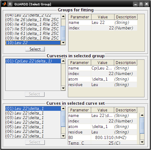
- Tutorial: Advanced Group creation
Tutorial Tasks
- Tutorial: Load data
- Tutorial: Basic Group creation
- Tutorial: Advanced Groupcreation (copy)
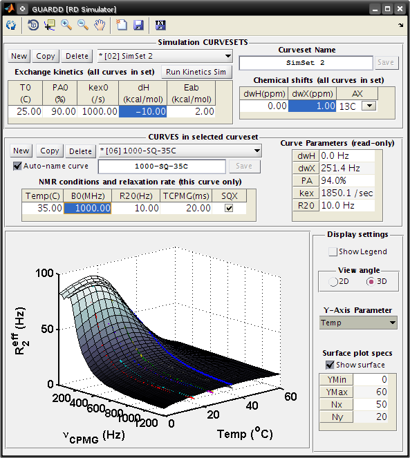
RD Simulator
Goal: Explore the nature of RD pheneomnea and create simulated Group data for planning experiments and edification
- Tutorial: Data simulation
Key sections of code
SimulationCurve.m
- holds a single curve for GUARDD simulation
SimulationCurveset.m
- holds a single curveset for a GUARDD simulation
SimulationSession.m
- holds information for all simulations in GUARDD
Kinetic Simulator
Goal: Explore the nature of two-state exchange phenomenea for planning experiments and edification
- Tutorial: Kinetic simulation
- See related: Kinetic simulation equations are covered later in this Manual
GUARDD Analysis menu
Fit Dispersion
Goal: Implement fits to Group, view results, log notes, and designate parameter validity
- The “product” is a best fitResult, and its parameters which are OK (those are used/displayed in subsequent analyses)
- Note: Tasks completed in this window are automatically committed (no need for an “OK” or “Save” command)
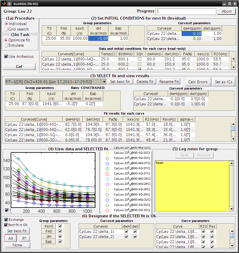
- This window contains six panels for fitting tasks
- Panel: (1a) Procedure
- Individual → Specify one set of initial conditions for one simulation or optimization
- Grid search → Specify a range of initial conditions for many simulations or optimizations
- Panel: (1b) Task
- Optimize fit → Starting at the initial conditions, iteratively alter parameter to minimize the χ2 for the Group, read [Manual#Fitting_data here]
- Simulate → Simulate the initial conditions for the fit
- Useful for seeing what the initial conditions look like
- Checkbox: Use Arrhenius → Use Arrhenius relation with ΔH and EAB for temperature-dependence of kex and PA
- Button: Go! → Initiate task
- Panel: (2) Set INITIAL CONDITIONS
- Note: The initial value of R20 for each Curve is set to Min(2Eff) for that Curve
- This panel operates in (Individual) or (Grid Search) mode, determined by Panel (1a)
- (Individual)
- Table: Group parameters → The kinetic parameters apply to the entire Group
- Table: Curveset parameter → The structural parameter apply to each Curveset
- Table: Data and initial conditions for each Curve (read-only) → Summary of dataset and its initial fit conditions
- Grid Search
- Table: Grid search → Limits of each dimension in grid search
- Panel: (3) SELECT fit and view results
- List → Select one of the available fits
- The fit name is automatically generated from 5 features
- FIT vs SIM: Designates whether the fitResult is for an optimization (FIT) or simulation (SIM)
- -1 vs -G: Designates whether the fitResult is from an individual fit (-1) or from a grid search (-G)
- [–] vs [CR]: Designates whether the Arrhenius “constrain rates” option is off (–) or on (CR)
- Chi2=###: Designates the value of χ2 for the Group (lower value is better fit)
- [Date-Time]: Designates the date and time at which the fitResult was created
- Button: Set best fit → Designate the current fit as the best one, which is displayed in all appearances of Group parameters
- Button: Delete fit → Remove the selected fit from the list
- Button: Rename fit → Rename the currently selected fit
- Useful for when certain constraints are used, or if it is selected from a grid
- Button: Calc Errors → Initiate Monte Carlo error analysis on the Group
- Button: Set as ICs → Set the current fitResult as the initial conditions for the next fit
- Useful for altering fit conditions during user-directed optimization
- List → Select one of the available fits
- Panel: (4) View data and SELECTED fit
- (Self explanatory)
- Panel: (5) Log notes for Group
- These can be displayed in the Notes window
- These can be exported in the Results Table window
- Panel: (6) Designate if SELECTED fit is OK
- To display/analyze a given best fit parameter, the best fit must be OK AND the particular parameter must be OK
- Checkbox: Exchange: The Group exhibits exchange (true/false)
- Checkbox: Best fit is OK: The Group fit is OK, which is required for subsequent display of fit results (true/false)
- Button: Set best fit → Designate the current fit as the best one, which is displayed in all appearances of Group parameters
- Button: All → Mark all the parameters as OK
- Button: R → Make only R20 and Rex as OK
- Button: None → Mark all of the parameters as NOT OK
- Tutorial: Basic fitting
- Tutorial: Multi-temperature fitting
- Tutorial: Multi-temperature + multi-Curveset fitting
- See related: fitting equations
- See related: minimizing χ2
Batch Task
Goal: Queue up lengthy computations for sequential processing
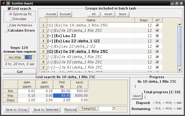
- Tutorial: set up a batch task
Notes
Goal: Document notes on Session, and read notes on all Groups
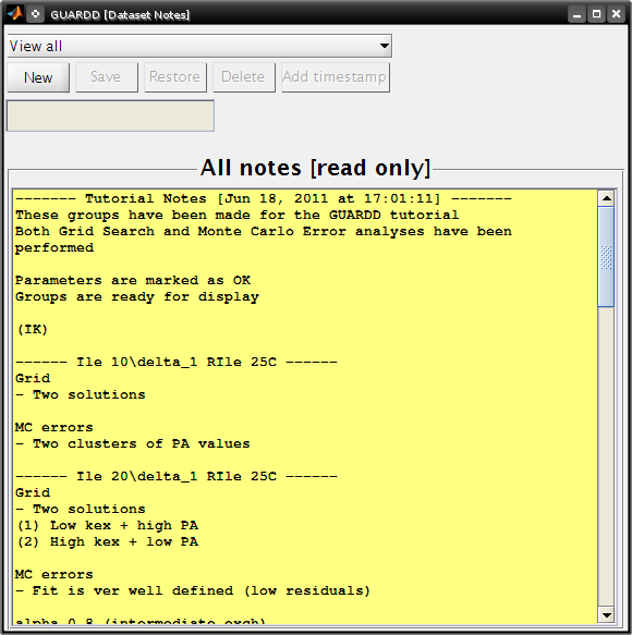
- Group notes can be modified in the Fit RD window
- Group notes can be read and exported to plain-text in the Results Table
- Tutorial: View notes for organization
Debug
- Runs the code in the function GUARDD.m/menu_run_code_Callback(), used for debugging
- Helpful for debugging features of GUARDD
GUARDD Output menu
Save session
Goal: Write the session to MATLAB file to save data and program state
Display Dispersion
Goal: Display RD Curves in a Group to assess fit quality (via residuals) and prepare figures for dissemination
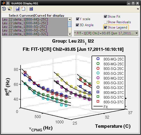
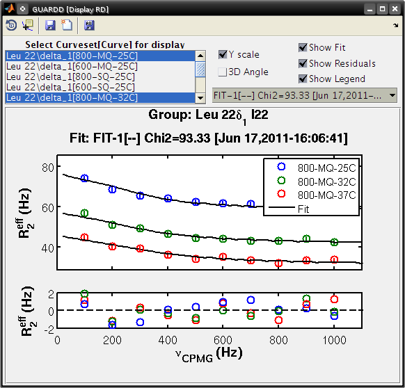
- Tutorial: display the dispersion
Display Chi2 Map
Goal: Browse the results of a grid search or MC error analysis to assess and refine fit
- Key info on features of chi2 maps
- The χ2 map is a hypersurface with amplitude χ2
and one dimension for each independent fitting parameter
- E.g., 14 parameters yields a 14D hypersurface
- Lower value of χ2 indicates a more precise fit to the data
- The goal is to obtain paramters at the global minimum of χ2
- Issue: the nonlinear nature of RD yields a “rough” χ2 map that can trap the fitting routine in local minima
- The χ2 map is a hypersurface with amplitude χ2
and one dimension for each independent fitting parameter
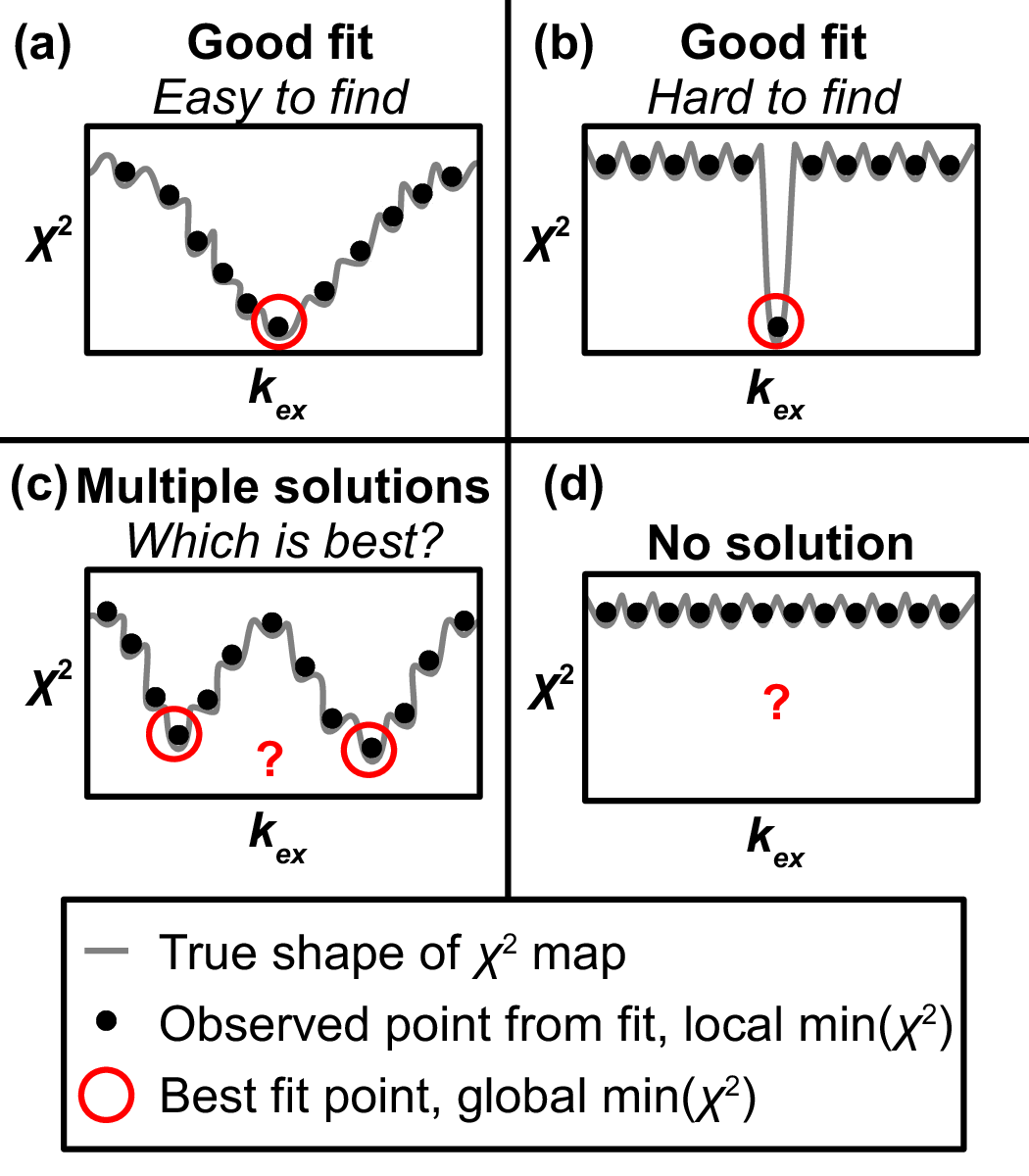
Figure above The response of χ2 to just one parameter kex produces a 2D slice through the hypersurface to illustrate four commonly encountered shapes that pose distinct challenges in obtaining an accurate fit.
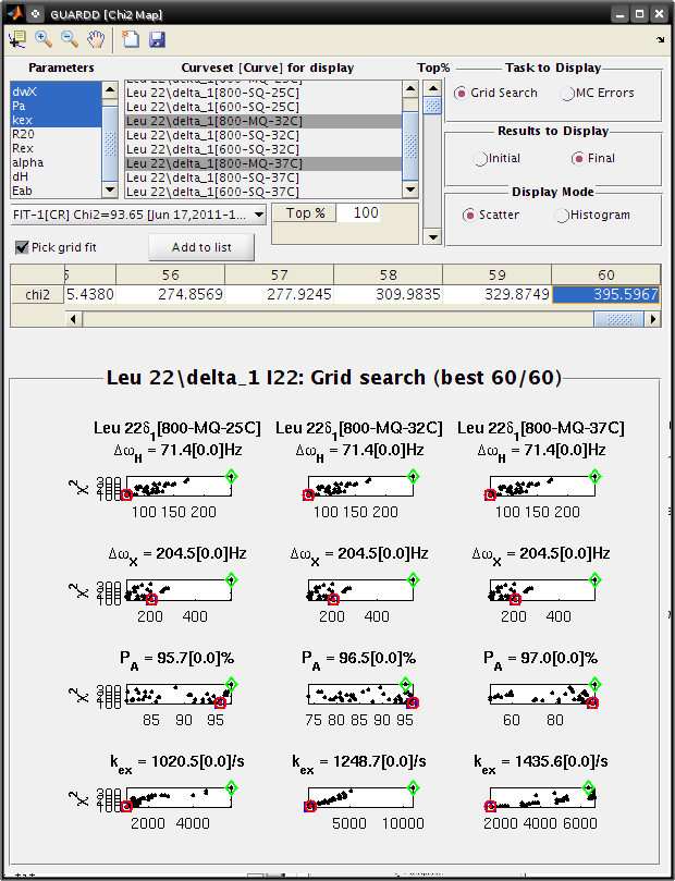
Goal: Interpret the Grid Search results the Chi2 Map window
- Each subplot shows a single parameter on the X-axis, and its different values in different fits
- Each black point corresponds to ONE optimized fit result
- There are 60 fits in this example (hence 60 points in each subplot), each of which started from a different location in parameter space
- Those initial locations can be displayed by setting Results to display: Initial
- The red circle designates the currently selected fit result
- The blue square designates the best fit from the grid search
- Clicking Pick grid fit will allow selection of any of the grid fits shown
- The green diamond designates the currently selected fit from the displayed grid list
- Any of these can be added to the list of fits, if desired
- Initial conditions sampled from the grid search are uniformly
distributed across paramter values
- This is shown by selecting Initial conditions and Histogram mode
- Tutorial: View grid search results for a good fit
- Tutorial: View grid search results for a bad fit
- See related: grid search; covered later.
Select fit from grid search
Goal: To examine a particular fit from the grid search that is not the minimum χ2, it must be selected from the list. This is helpful for checking another well in χ2 space.
- Tutorial: select fit from grid search
Display Monte Carlo Errors
Key info on Monte Carlo analysis
- The goal of MC analysis is to generate and fit many synthetic datasets which differ from one another by an amount related to the goodness of fit to the original data
- Each synthetic dataset will have a different set of optimal fit values (e.g., PA, kex)
- The distribution of fitted values reflects the degree to which the original data define its own optimal values - Example: A worse optimal fit to the original data yields more different MC datasets and therefore more different optimal parameter values
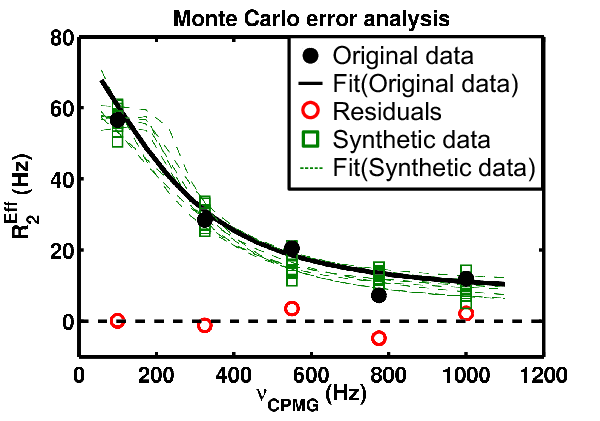
Figure above The example data contains 5 observations (black), 5 residuals (red), and 10 synthetic datasets (green squares), each with their own fit (green dotted lines) and set of optimized parameter values
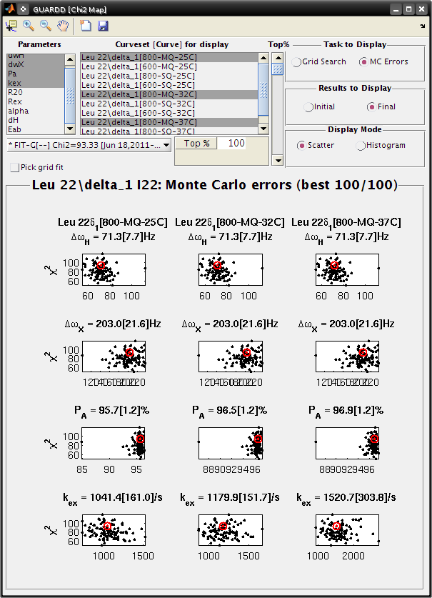
Goal: Interpret the MC Errors results the Chi2 Map window
- Eachsubplot shows a single parameter on the X-axis, and its different values in different fits
- Each black point corresponds to ONE optimized fit result to a synthetic MC dataset
- There are 100 fits in this example (hence 100 points in each subplot), each of which corresponds to a synthetic MC dataset
- The initial conditions to each fit are given by the best fit to the original data (see Results to display: Initial)
- The red circle designates the best fit to the original data
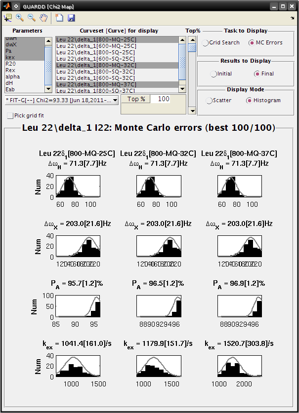
- Set Display Mode: Histogram
- The gray lines show the hypothetical distributions reflecting “errors” in the data
- The mean of each distribution is from the best fit value to the original data
- The standard deviation of each distribution is the standard deviation from the distribution of MC fitted values
- Each deviation is reported as the “error” in each fitted parameter (shown in brackets)
- Note: it is usually best to use a Top%=100% for MC errors
- Sometimes anomalous fits yield very large χ2, and can be discarded, but this is rare
- Tutorial: View Monte Carlo results for a good fit
- Tutorial: View Monte Carlo results for a bad fit
- See related: Monte Carlo error estimation
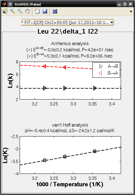
Display rates
Goal: Display results of rate analysis using Arrhenius and vant Hoff relations
- Tutorial: view the rates
- See related: Arrhenius equations
- See related: vant Hoff equations
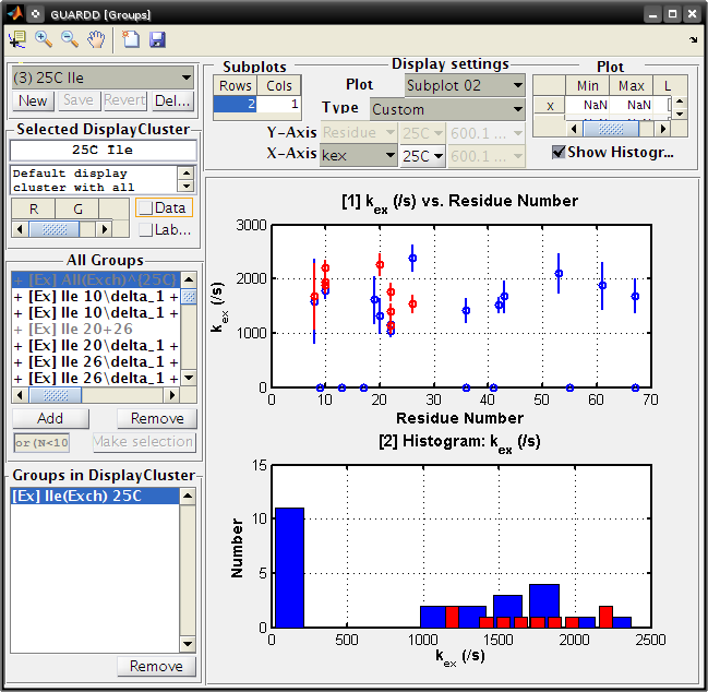
Display group results
Goal: Visually organize fitting results to seek the nature of molecular motions
- Button: New → Add new empty DisplayCluster to hold Groups for displaying results
- Panel: All Groups → Lists all Groups available to add/remove to/from the selected DisplayCluster
- Button: Make selection → Deprecated function to intelligently select Groups from GUARDD
- Panel: Groups in DisplayCluster → Lists all Groups in the selected DisplayCluster (can be removed)
- Panel: Display Settings
- Table: Subplots → Used to create a set of subplots for the display
- Plot number → Select the subplot number (From 1 to Nrow*Ncol)
- Type → Select plot type (Custom will allow for any parameters to be displayed, others are pre-arranged)
- Y-Axis → Select what to be displayed on Y-axis (non-histogram only)}
- X-Axis → Select what to be displayed on the X-axis
- Table: Plot limits → Set NaN for auto-limits, or type in your own and use linear or log scale (applies to all subplots, sorry!)
- Checkbox: Show Histogram → Shows the histogram (requires only X-axis values)
- Notes
- Some paramters plot one point per Group (e.g., PA or kex(37C))
- Some parameter plot one point per Curveset (e.g., |ΔωX|) and hence multiple points per Group
- Some paramters could plot one point per Curve (e.g., Rex) but the FIRST Curve is selected by default
- Otherwise there would be too many points on the plot
- Tutorial: View display results in cluster
Key sections of code
DisplayCluster.m
- Holds information on the name, color, and Groups for display
ParamDisplay.m
- Holds information for display of the parameters (subplots, X and Y content)
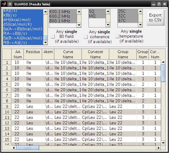
Display results table
Goal: Produce table of results for easy browsing
- Notes
- Table is dynamically generated based on the user’s selection
criteria from an arbitrary set of RD parameters and Curves
- E.g., only PA and kex at one temperature, instead of all RD parameters for all Curves for all Groups
- This customized table can be exported to plain-text for publication or external analysis
- Table is dynamically generated based on the user’s selection
criteria from an arbitrary set of RD parameters and Curves
- Button: Export to CSV → creates two plain-text files (two-column
format and one-column format)
- One is easier for plotting in external programs
- Another is easier for preparing a publication quality table
- Tutorial: display results table
Tips for optimal use
Program tips
- Save frequently
- Drawing windows is relatively slow
- Use the main display window to only update displays of interest
- Use a CPU monitor application to see when GUARDD is processing
results (e.g., fitting, drawing windows, exporting files) - Do not make other changes when performing grid search or error estimates - Data can be viewed but not altered - This is because data structures are stored before the batch run (or a single grid search or single error estimation) then re-saved upon completion of a batch step or single grid search or single error estimation
Fitting tips
Usually, dispersions with larger Rex have a more well-defined solution. Small Rex and/or noisy data are usually accompanied by challenges in fitting
- If unsure about the fit, then don’t interpret fitted parameters
quantitatively
- Additional inaccurate information can obscure proper interpretation of dynamics
- A poor fit to the two-state model may indicate more complex exchange, such as three-state
- Note this residue, and consider other fitting equations or more complex exchange models (unfortunately, not available in GUARDD v.2011.09.11)
- Three solutions for ill-defined fits
- Select one of the fits, but mark the ill-defined parameters as “Not OK,” thus preventing their mis-interpretation in subsequent analyses.
- Alter the Group and re-fit. One may remove noisy Curves and/or add additional Curvesets to help constrain the values of kex and PA.
- Acquire more data and re-fit the new Group. The RD Simulator can help determine optimal conditions of temperature, magnetic field strength, and/or quantum coherence for efficient use of spectrometer time.
- Check for outliers in fitted data
- Check sequence mapping for outliers
- Check χ2 and fits for those outliers
- What type of exchange do proximal residues exhibit?
- Make sure fits which show no exchange have “NoEx” model selected as best
- Check neighboring residues
- Check dispersions for neighboring residues to get an idea of the type of motions one may expect in that region of the structure
- If there is concerted motion, then kex and PA (and their temperature-dependence Ea(A → B), Ea (B → A), dH, dS) will be the same (or close) for residues close in structure
- Note: There is no requirement that neighboring residues be similar though
- kex is most sensitive fitting parameter
- Use the largest number of grid search steps
- kex should increase with temperature (e.g., Arrhenius)
- PA may increase (ΔH < 0), decrease (ΔH > 0) or remain constant (ΔH=0) with temperature
GUARDD approach to fast exchange and PhiEx
Issue: In fast exchange (kex >> Δν = Δω / (2π)), the quantities PA, PB and Δω are correlated, and therefore cannot be independently defined
- Solution: sometimes although neither quantity can be defined independently, the quantity ΦexX = PAPBΔωX2 = PA(1-PA)ΔωX2, where X refers to the X nucleus, can be well-defined (Luz, 1963; Ishima, 1999)
- Examine ΦexX in the Chi2 Map window to help assess the
sensitivity of the final fit to either initial conditions (via grid
search) or to noise in the data (via Monte Carlo error estimation)
- In some cases, the parameters PA and ΔωX are relatively sensitive to initial conditions (wide χ2 maps), whereas Φex is relatively less sensitive (more narrow χ2 map), which may indicate that it is reasonable to interpret Φex, but not PA.
- The Chi2 Map window displays a correlation plot of the optimized values of ΔωX2 and PAPB. In fast exchange, a strong correlation between these parameters yields a line of points, facilitating detection of fast exchange.
- Check for fast exchange via the Fit RD window by comparing values of kex and Δω as well as the exchange parameter α, which indicates fast exchange in the range 1.0 to 2.0 (Millet et al., 2000).
Limitations
Liabilities of linkage to MATLAB
- GUARDD is slower than if it were coded using C or Python, for example
- MATLAB is an interpreted language
- Graphical interface uses Java
- Drawing the display, while reading or writing large session files, or while fitting data
- Malfunctions in MATLAB may hinder functionality of GUARDD
- However, enhancements to MATLAB may imbue enhancements to GUARDD
- User must have access to MATLAB (i.e., GUARDD is not a standalone program)
- However, MATLAB is a convenient cross-platform solution for dissemination of software
- Cannot be run using Octave, which can run many other MATLAB programs
- Octave does not support the graphical user interface that is a key feature of GUARDD
- For what its worth, Octave supports a distinct GUI library called “Zenity”
Limitations of GUARDD functionality
- Exchange model is restricted to two-state using the all-timescales MQ Carver-Richards-Jones formulation
- No simplifications assuming skewed populations (PB < PA) (Ishima, 1999)
- No simplifications assuming fast-exchange (kex > Δν)
- No three-site exchange
- No ZQ or DQ coherences
- No pressure-dependence of RD
- No Anti-TROSY/TROSY analysis
- No temperature-dependence via transition state theory
- No error analysis options: jacknife, covariance matrix method
Computational procedures
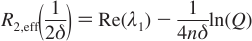
Convert NMR signal intensity to relaxation rate
Goal: Given NMR signal intensites, generate a relatxation Curve
- Input
- I(νCPMG) = signal intensity in the 2D spectrum acquired with refocusing frequency νCPMG
- I0 = reference signal intensity obtained in the spectrum with no refocusing block
- TCPMG = duration of the refocusing block
- Output
- R2Eff
- Errors in intensities σ(R2Eff) are estimated via standard deviation from repeat measures of I(νCPMG)
R2Eff = -ln( I(νCPMG)/I0) / TCPMG
Converting ppm to rad/s
Goal: Obtain rad/s quantity for chemical shift difference using ppm value * Note rad/s is requried for trigonometric functions, like tangent
Note: Hz = /s is useful for direct comparison to kex (also in /s) in determining exchange timescale
- Input
- ωX (rad/s)
- γX (from nucleus identity)
- B0
- Output
- ωX(rad/s) = 2πB0γXωX(ppm)
- νX(Hz) = B0γXωX(ppm)
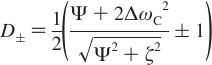
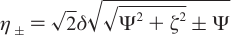
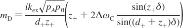
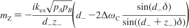
Carver-Richards Jones for MQ disperstions
Goal: Obtain dispersion Curve R2Eff as a function of νCPMG given a set of 5 parameters
- Input
- ΔωH
- ΔωX
- PA
- kex
- R20
- νCPMG
- Process
- δ = 1 / (4νCPMG)
- n = TCPMGνCPMG
- Note: MQ simplifies to SQ if ΔωH = 0
- (See equations below)
- Output
- R2Eff
- Location in code
chi2_MQRD_CRJ_group.m
chi2_MQRD_CRJ.m
- Reference
- Korzhnev (2004)


Fitting data
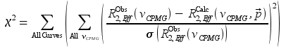
Goal: Obtain a set of parameters that accurately describe RD Curves in the Group Goal: Minimize the sum of squares target function
Input
- R2EffObs = RD Curve data points
- σ(R2EffObs) = Errors in RD Curve data points
- Curve condition: B0
- Curve condition: Temperature
- Curve condition: QC
- Curve condition: AX
- Curve condition: TCPMG
- Fitting parameters: p
- PA and kex for each temperature
- |ΔωH| and |ΔωX| for each Curveset
- R20 for each Curve
Process
- MATLAB fmincon iteratively alters the fitting parameters
p to minimize the target function χ2
- R2Calc = calculated point using the Curve conditions and the independent fitting parameters p for the Group
- χ2 becomes smaller as the Curve fit more closely matches the observed data
Output
- χ2
Location in code
FitResult.fitMe
Exchange broadening
Goal: Estimate exchange broadening Rex (height of the dispersion Curve) using the fitted RD Curve
- Input
- Process
- Sometimes evaluation at 0 Hz is not valid, therefore try 1 Hz, then2 Hz, …
- Try to use νCPMG values as close to 0 and infinity as possible
- Output
- Rex
- Location in code
FitResult.analyzeMe()
calculate_Rex.m
Rex ~ R2EffFit(νCPMG~0 Hz) - R2EffFit(νCPMG ~104Hz)
Exchange timescale alpha
Goal: Estimate scaling factor α for time regime of chemical exchange
Input
- Rex at at least two field strengths
- Δω at the same field strengths
Output
- α
- 0 <= α < 1 Slow exchange
- α = 1 Intermediate exchange
- 1 < α <= 2 Fast exchange
Location in code
FitResult.analyzeMe()
calculate_alpha.m
- Reference
- Millet, et al. (2000)
α = d( ln(Rex) ) / d( ln(Δω) )
Exchange quantity PhiEx
Goal: Calculate quantity Φex that appears in fast-exchange approximation to RD equations
Sometimes this quantity is well-defined despite correlated/ill-defined PA and Δω
- Input
- PA
- ΔωX where X is the X nucleus
- Output
- ΦexX (Hz2)
- Location in code
FitResult.analyzeMe()
- Reference
- Luz & Meiboom (1963)
- Ishima & Torchia (1999)
ΦexX = PAPBΔωX2 = PA(1-PA)ΔωX2
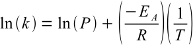
Arrhenius: Determining activation energy
Goal: Obtain activation energy and pre-exponential rate to characterize temperature-dependence of rate
- Input
- PA at 2+ temperatures
- kex at the same temperatures
- Process
- R = gas constant
- T = absolute temperature
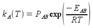
- k = kA = (1-PA)kex (or kB = PAkex) = kinetic rate of exchange from A→B (or B→A)
- Errors from MATLAB’s fit routine (provided data at more than two temperatures), or from propagation of relative error from the fitting variables (when limited to data at only two temperatures).
- Output
- P = PAB (or P = PBA) Pre-exponential rate, the exchange rate from A→B (or B→A) at infinite temperature
- E = EAB (or E = EBA) = Activation energy (≈ enthalpy) required to exchange from A→B (or B→A)
- Location in code
RateAnalysis.analyzeMe
- Reference
- Winzor & Jackson (2006)
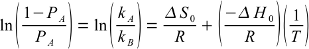
vant Hoff: Determining enthalpy
Goal: Obtain exchange enthalpy and entropy to characterize temperature-dependence of population
- Input
- PA at 2+ temperatures
- Process
- R = gas constant
- T = absolute temperature
- K = (1-PA) / PA = kA / kB = equilibrium constant for exchange
- Errors from MATLAB’s fit routine (provided data at more than two temperatures) Or from propagation of relative error from the fitting variables (when limited to data at only two temperatures).
- Output
- ΔS = system entropy change from A→B
- ΔH = system enthalpy change from A→B
- Note: Entropy is unreliable since it is highly sensitive to relatively noisy input data
- Location in code
RateAnalysis.analyzeMe
- Reference
- Winzor & Jackson (2006)
Kinetic simulator
Goal: Itemizes all kinetic parameters of interest for two-state exchange, given minimal input required
- Input
- ΔH
- EAB
- kex0 = kex(T0)
- PA0 = PA(T0)
- T0 is an arbitrary temperature
- Process
- R = gas constant
- T = absolute temperature
- (See below)
- Output
- ΔH
- ΔS
- EAB
- PAB
- EBA
- PBA
- kex(T)
- PA(T)
- kA(T)
- kB(T)
- T is an arbitrary temperature
- Location in code
SimulationCurveset.setKineticSpecs

SimulationCurveset.calc_PA

SimulationCurveset.calc_kA

SimulationCurveset.calc_kex

SimulationCurveset.calc_kB
- Reference
- Winzor & Jackson (2006)
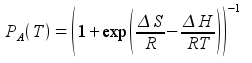
Using ΔH and PA(T0), the van’t Hoff relation yields ΔS
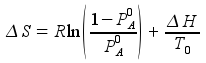
which, with ΔH, determines PA at any temperature via van’t Hoff
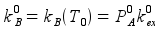
Next, using PA and kex at T0 determines kA and kB at T0
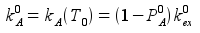
and using EAB and kA at T0, the Arrhenius relation yields PAB
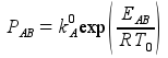
which, with EAB, yields kA at any temperature via Arrhenius
Next, knowledge of PA and kA at any temperature yields kex at any temperature
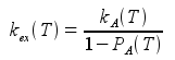
and therefore kB at any temperature
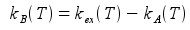
Knowledge of kB at any temperature yields EBA via the Arrhenius relation and selection of any two temperatures T1 and T2 (e.g., 280 K and 320 K)
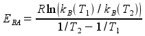
Finally, using kB(T0) and EBA, the Arrhenius relation yields PBA
Grid search
Motivation: Nonlinear nature of RD phenomena makes the relationship between χ2 and fitting parameters (p) difficult to predict * Optimization algorithms often “fail” by finding a local minimum of χ2, which is sensitive to initial fitting conditions, instead of the intended global minimum of χ2
- Goal: Fit data multiple times to assess sensitivity of final fit
- to initial conditions
- Six-dimensional (6D) grid search
- |ΔωH|
- |ΔωX|
- PA0 = PA(T), where T is a specified temperature (e.g., 25C)
- kex0 = kex(T0), where T0 is a specfied temperature (e.g., 25C)
- EAB (only for consraining rates via Arrhenius)
- ΔΗ (only for consraining rates via Arrhenius)
- Each point specifies initial conditions for the fit, as follows
- Δω values are used for every Curveset in the Group
- Note: this may be sub-optimal since each Curveset can have a different Δω value
- If constrain rates is NOT used
- PA0 is used for all temperatures in the Group
- kex0 value is used at temperature T0 and increased by 2x for each increase in 10C from T0 (i.e., kex(T) = kex0(T-T0)/10)
- If constrain rates IS used
- PA(T) determined using PA0and ΔH
- kex(T) determined using kex0and EAB
- R20 is always the minimum value of the observed R2 in the Curve
- Δω values are used for every Curveset in the Group
Recommendations on bounds at T0 = 25C
| Iteration | ΔωH(ppm) | ΔωΧ(ppm) | PA0(%) | kex0(/s) | EAB (kcal/mol) | ΔH (kcal/mol) |
|---|---|---|---|---|---|---|
| Min | 0.01 | 0.1 | 70 | 500 | -20 | -20 |
| Max | 0.2 | 3 | 99.9 | 3500 | 20 | 20 |
| Steps | 1-3 | 2-5 | 2-10 | 3-10 | 2-5 | 2-5 |
Recommendations on number of steps
| Group Size | Num(Curves) | Num(Steps) | Notes |
|---|---|---|---|
| Small | 1-5 | 5-50 | Easy to fit, usually only one solution |
| Medium | 5-10 | 20-100 | Usually easy to fit, few solutions |
| Large | 10-20 | 100-200 | Sometimes challenging, several solutions |
| Very Large | 50-100 | 500+ | Very challenging to fit |
- Unsorted notes
- kex seems to be a very sensitive parameter, use the most points here
- Sometimes MATLAB does not alter Δω values for multiple Curvesets
- EAB and ΔH can be very difficult to optimize via grid search
- Location in code
Group.gridSearch
Monte Carlo error estimation
Motivation: The final fit to RD data are sometimes very sensitive to noise in the data
Goal: Generate and fit multiple synthetic data to assess sensitivity of final fit to noise in data
Monte Carlo procedure generates and fits synthetic data consistent with observed residuals (related to noise)
Procedure
- Calculate residuals for each νCPMG value in a given Curve
- ε(νCPMG) = R2EffObs(νCPMG) - R2EffCalc(νCPMG)
- The residuals are used to create a normal distribution for the Curve with mean and variance
- Norm(mean(ε), var(ε))
- Alternatively, the experimental errors σ(R2EffObs) can be used
- Norm(mean(σ), var(σ))
- Generate a synthetic dispersion Curve using the fit at each νCPMG plus a random sample from the distribution
- R2EffSynth = R2EffCalc(νCPMG) + Sample( Norm(mean(ε), var(ε)) ), or using Norm(mean(σ), var(σ))
- Repeat for each Curve in the Group such that a synthetic Group is produced
- Fit the synthetic Group using initial conditions from the best fit of the actual data.
- Repeat (3)-(5) multiple times (default 100x, can be changed in settings “Nmc”)
This yields 100 synthetic Groups and 100 sets of optimized fit parameters
- Calculate the error in a given parameter as the standard deviation of the optimized fit parameter from its 100 element distribution
- Errors in subsequent quantities (e.g., kA, kB ln(kA), etc.) are estimated using propagation of error assuming all parameters are uncorrelated (zero covariance)
Notes
- Number of MC error iterations can be set via
Input…Settings…Nmc
- Debugging output can display the fits to each data via
Input…Settings…OUTPUT_DEBUG_ERRORS
Location in code
FitResult.calculateErrors
Reference
- Motulsky (2003), p. 108
Glossary
- AX: Any nucleus with mass number A and chemical symbol X (e.g,. 1H, 13C, 15N)
- B0: Magnetic field strength (Tesla)
- C: Curve number within the curveset
- Chi2: χ2; Goodness of fit metric (smaller value indicates better fit)
- CPMG: Carr-Purcell Meiboom-Gill (four scientists who poineered relaxation dispersion methods)
- CS: Curveset number
- CTOT: Total curve number within the group
- Curve: A single set of R2Eff(νCPMG) data points
- Curveset: Designates a ΔωH and ΔωX to a set of one or more Curves
- DQ: Double Quantum (not implemented in GUARDD)
- EAB: EB - EA; Activation energy to exchange from A→B (cal/mol)
- G: Group number
- Group: Designates a PA and kex at each temperature for a set of one or more Curvesets
- GUARDD: Graphical User-friendly Analysis of Relaxation Dispersion Data
- GUI: Graphical User Interface
- kA: (1-PA)kex; Rate of exchange from A→B
- kB: PAkex; Rate of exchange from B→A
- kex: kA + kB; Total exchange rate between states (/s)
- MC: Monte Carlo (randomization method used here for error analysis)
- MQ: Multiple Quantum (signal detected in NMR); Note: MQ RD curves are sensitive to both ΔωH and ΔωX
- NMR: Nuclear Magnetic Resonance
- NMR probe: One nucleus in the target molecule that can be observed via NMR; designated a unique unique residue number (e.g., 1,2,3,…) and atom (e.g,. HN, CO, Cδ2)
- PA: Populationfraction of A state (fraction, %)
- ppm: Parts Per Million (a dimensionless unit of measure for relative comparison)
- R: Gas constant
- R20: Transverse relaxation rate in the absence of exchange (Hz)
- RD: Relaxation Dispersion
- SQ: Single Quantum (signal detected in NMR); Note: SQ curves that pulse on AX nucleus are sensitive only to ΔωX (ΔωH is fixed to zero)
- TCPMG: Total duration of the CPMG block in the NMR RD experiment
- ZQ: Zero Quantum (not implemented in GUARDD)
- γX: Gyromagnetic ratio for nucleus X (MHz/Tesla)
- ΔH: HB - HA; Enthalpy difference to exchange from A→B (cal/mol)
- Δν: Chemical shift difference in Hz
- ΔωH: 1H chemical shift difference between states A and B (ppm, rad/s) - MQ only
- ΔωX: AX chemical shift difference between states A and B (ppm, rad/s)
- νCPMG: Precession frequency of refocused magnetization during CPMG period of NMR RD experiment
References/Further Reading
Please cite your usage of GUARDD in BOTH ways
- Kleckner, I. R., & Foster, M. P. (2012). GUARDD: user-friendly MATLAB software for rigorous analysis of CPMG RD NMR data. Journal of biomolecular NMR, 52(1), 11–22.
- http://code.google.com/p/guardd/
Review on protein dynamics via NMR
- Kleckner, I. R., & Foster, M. P. (2011). An introduction to NMR-based approaches for measuring protein dynamics. Biochimica et biophysica acta, 1814(8), 942-968. Elsevier B.V. doi: 10.1016/j.bbapap.2010.10.012.
Fitting RD data is poorly determined
- Kovrigin, E. L., Kempf, J. G., Grey, M. J., & Loria, J. P. (2006). Faithful estimation of dynamics parameters from CPMG relaxation dispersion measurements. Journal of magnetic resonance (San Diego, Calif. : 1997), 180(1), 93-104. doi: 10.1016/j.jmr.2006.01.010.
- Ishima, R., & Torchia, D. a. (2005). Error estimation and global fitting in transverse-relaxation dispersion experiments to determine chemical-exchange parameters. Journal of biomolecular NMR, 32(1), 41-54. doi: 10.1007/s10858-005-3593-z.
Fast exchange approximation
- Luz, Z. & Meiboom, S. (1963). Nuclear magnetic resonance study of protolysis of trimethylammonium ion in aqueous solution - order of reaction with respect to solvent. J. Chem. Phys., 39, 366-370.
- Ishima, R. & Torchia, D.A. (1999). Estimating the time scale of chemical exchange of proteins from measurements of transverse relaxation rates in solution. Journal of Biomolecular NMR, 14, 369-72. [http://view.ncbi.nlm.nih.gov/pubmed/10526408]
MQ dispersion
- Korzhnev, D. M., Kloiber, K., & Kay, L. E. (2004). Multiple-quantum relaxation dispersion NMR spectroscopy probing millisecond time-scale dynamics in proteins: theory and application. Journal of the American Chemical Society, 126(23), 7320-9. doi:10.1021/ja049968b.
Quantum Coherences in dispersion
- Korzhnev, D.M., Neudecker, P., Mittermaier, A., Orekhov, V. Y., & Kay, L. E. (2005). Multiple-site exchange in proteins studied with a suite of six NMR relaxation dispersion experiments: an application to the folding of a Fyn SH3 domain mutant. Journal of the American Chemical Society, 127(44), 15602-11. doi: 10.1021/ja054550e.
Exchange timescale α
- Millet, O., Loria, J. P., Kroenke, C. D., Pons, M., & Palmer, A. G. (2000). The Static Magnetic Field Dependence of Chemical Exchange Line broadening Defines the NMR Chemical Shift Time Scale. Journal of the American Chemical Society, 122(12), 2867-2877. doi: 10.1021/ja993511y.
Nonlinear fitting
- P, B., & D, R. (2003). Data reduction and error analysis for the physical sciences. (D. Bruflodt, Ed.) (3rd ed.). New York, NY: McGraw-Hill.
- Motulsky, H. J., & Christopoulos, A. (2003). Fitting models to biological data using linear and nonlinear regression. A practical guide to curve fitting. (GraphPad Software Inc., Eds.) (2nd ed.). San Diego CA: GraphPad Software Inc.
Temperature-dependence of rate and equilibrium constants (Arrhenius and vant Hoff analyses)
- Winzor, D. J., & Jackson, C. M. (2006). Interpretation of the temperature dependence of equilibrium and rate constants. Journal of Molecular Recognition, c(August), 389-407. doi: 10.1002/jmr.