Tutorial

General notes

• Sample data for this tutorial is provided here.
• Tutorial images shown below are from GUARDD v.2011.07.01 and associated GUARDD-Session-Tutorial.mat file
• This tutorial is also compatible with GUARDD v.2011.09.11 and associated GUARDD-Session-Tutorial.mat file
• v.2011.09.11 session uses more points in grid search than the v.2011.07.01 session (150 vs. 60)
• See Manual for Glossary
• GUARDD utilizes multiple GUI windows (may need to be resized)
• Higher monitor resolution helps (1024x768 minimum)
• Matlab must remain open since it controls GUARDD
• GUARDD Main window must remain open since it controls other GUI windows
• Check Matlab command window for additional output
• GUARDD is sometimes slow. Turn on CPU monitor to see when program is processing
• Win: Ctrl+Alt+Del, click Task Manager, watch icon in task bar
• Mac: Applications folder → Utilities folder → launch Activity Monitor
• “Tooltips” are revealed by hovering mouse cursor over buttons, tables, etc

Download and unpack files

• Download Files here.
• Unpack files
  • E.g., /home/user/Desktop/ or C:My_Favorite_Folder\

Ensure proper directory structure

• GUARDD–YYYY.MM.DD/ (Note: YYYY.MM.DD codes for the date (e.g.,2011.06.17))
• There should also be a “tutorial” folder present, along with many .m and .fig files

Start GUARDD

• Start Matlab
• Open Matlab command window: Desktop…Command Window
• Navigate to GUARDD/ directory and start program
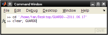
• Matlab command window:

cd c:\My_Favorite_Folder\GUARDD--YYYY.MM.DD\

• Note: YYYY.MM.DD is replaced by the date corresponding to the GUARDD version (e.g., 2011.06.08)
• To launch GUARDD, enter GUARDD in the command line:

clear; GUARDD

Important: Main window must remain open since it controls other GUI windows!

Check Matlab command window for additional output

Load data

Goal: Get Relaxation Dispersion data into the program for analysis

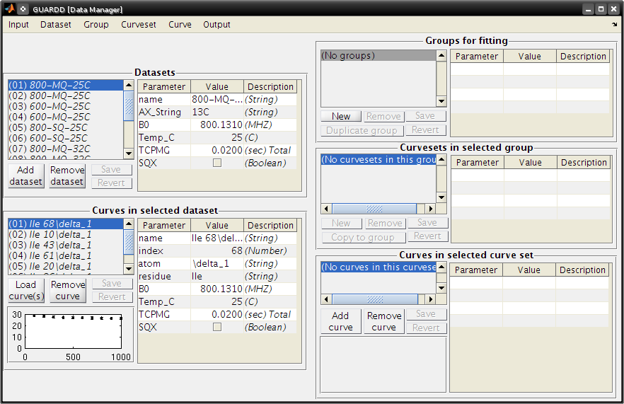
• From the Main GUARDD window, select the Input tab and click on Data Manager
• In the Data Manager window, select Input and click on Script
• Open the following file

tutorial/data/GUARDD-Data-ApoTRAP-Kleckner.txt

Note: There are two methods for importing your data to GUARDD

• Generate a data script
  • Each data script will adhere to the following format

NAME:        "The name for your dataset"
AX:          "Nucleus (e.g. 13C, 15N)"
B0:          "External field strength in units of MHz (e.g. 800.130981)"
TEMPC:       "Temperature in units of degrees Celsius"
TCPMG:       "CPMG time in units of seconds"
SQX:         "Boolean; set this to True if you're analyzing a single quantum dataset. Set it to False otherwise."
SETSPECS:    "This will set the previous specifications for the current dataset"

INDEX:       "The identifier for the NMR signal. This is ideally a number (e.g. 26 if the signal corresponds to Ile26)"
ATOM:        "The atom being analyzed (e.g. NH, CO, \delta_1)"
Residue      "Three letter code for the amino acid being analyzed (e.g. Ile for Isoleucine)"
OBS          VCPMG           R2              ERROR

• OBS, VCPMG, R2 and ERROR are columns containing data from your CPMG experiment.
• OBS will turn observation mode on and is required. This column should be numbered 1 through N where N is the number of data points recorded
• The VCPMG column should contain your CPMG pulse frequencies
• R2 should contain your observed R2 values at each CPMG frequency
• ERROR is optional - this column should contain the errors, if known, for each measured R2 value.
• Example data script: tutorial/data/GUARDD-Data-ApoTRAP-Kleckner.txt

• An nlin.tab file from NMRPipe (containing your peak information) and a vcpmg.txt file (containing your CPMG pulse frequencies) may be used.
• Examples…
  • tutorial/data/example_files/TRAP-SteApo-A26I-25C-800MHz-MQ-14ppm-nlin.tab
  • tutorial/data/example_files/TRAP-SteApo-A26I-25C-800MHz-MQ-14ppm-taufile.txt

14 datasets loaded

• 600 and 800 MHz
• 25, 32, and 37^oC
• SQ and MQ coherence

Create groups for fitting

• Goal: Aggregate RD curves from the same NMR signal (assignment) for group fitting

Essential notes on data organization

• Datasets designate experimental conditions
• Datasets contain Curves, which contain RD data
• Curves are aggregated across common NMR probes (assignment) into Curvesets (to share Δω values)
• Curvests are aggregated across different NMR probes into Groups (to share k_ex and P_A)
• Details regarding data organization are discussed in the Manual
• Open the Data Manager window
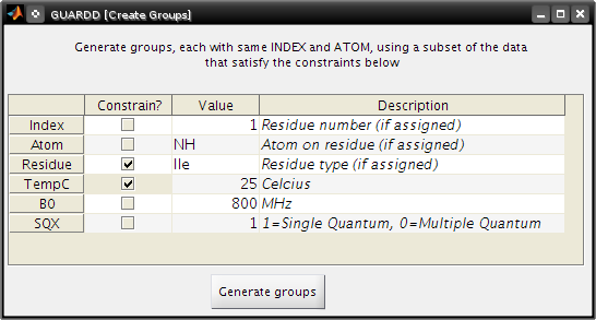
• Select the Group tab and click on Generate from subsets of data
• Create Groups

• Make groups only for Ile residues at 25^oC
• Check Residue
• Type Ile
• Check TempC
• Type 25

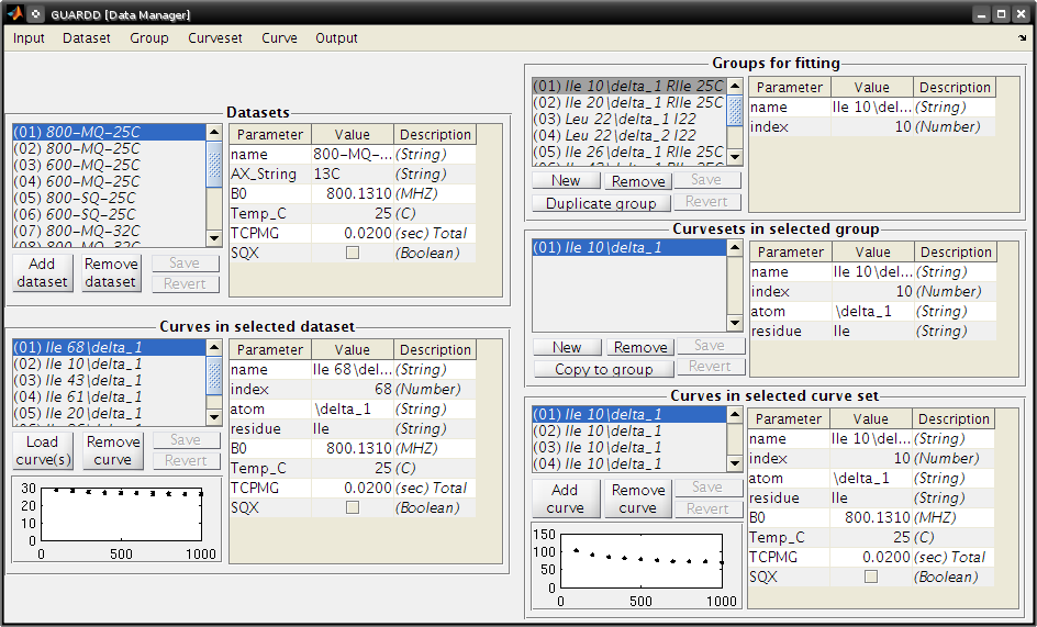
• Click Generate Groups

Data Manager

Group…Generate from subset of data…

• Create Groups
• Make groups only for index 22

• Check Index
• Type 22
• Click Generate groups

Data Manager

• Select the Group tab and click on Sort Groups
• Close the Data Manager window

Select groups that exhibit exchange

• Goal: Determine which groups exhibit flexibility, and therefore warrant further analysis
• For details, read more about describing dispersions in the Manual

Select Groups

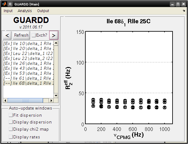
• In the Main window, click the Refresh button to show loaded groups
• Use < and > to cycle through groups
• Check Exch? if the data are not horizontal (i.e., if R_ex > 0)
• Note: all residues exhibit exchange except Ile 61δ₁ and Ile 68δ₁

Fit RD data

Goal: Obtain best-fit values for the 4-5 parameters required to describe each curve

• Δω_H = ¹H chemical shift difference between states A and B (ppm, rad/s, Hz) - MQ only
• Δω_X= ^AX chemical shift difference between states A and B (ppm, rad/s, Hz)
• P_A = Population fraction of A state (fraction, %)
• k_ex = k_A + k_B = Total exchange rate between states (/s)
• R₂⁰ = Transverse relaxation rate in the absence of exchange (Hz)

Fit simple group manually

Goal: Use Fit RD window to manually fit one group

• Determine optimal P_A and k_ex at each temperature (x1) → propagate to all curves in group
• Determine optimal Δω_H and Δω_X for each curveset (x1) → propagated to all curves in curveset
• Determine and R₂⁰ for each curve (x4)

Goal: Demonstrate basic fitting options (Simulate vs. Optimize, Individual vs. Grid)

• Details: Read more about the Fit RD window in the Manual

Fitting

• In the Main window: check the Fit Dispersion box

• Select Ile 26

• In the Analysis tab, click Fit RD

• The Fit RD window contains 6 panels for sequential fitting tasks

• (1a) Procedure: Individual

• (1b) Task: Simulate

• (2) INITIAL CONDITIONS: (Leave default)

  • Note: Often, one may change starting P_A, k_ex,

  Δω_H, and Δω_X - To change starting R20, see https://groups.google.com/d/topic/guardd/A4c-3bn21Yk/discussion

• Click Go! (1-5 sec)

  • Note that these initial conditions are reasonable (fit is somewhat close to data)

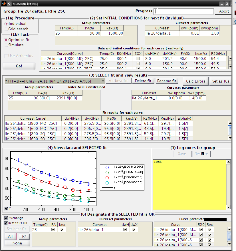
• (1b) Task: Optimize fit

  • Click Go! (5-30 sec)

• (3) SELECT fit and view results

• There are three “fits” to the data: NoEx, Sim-1, and Fit-1

• Select each at a time, and note that Fit-1 is the best (lines go through data in panel (4))

• Select Fit-1

• Click Set best fit

• (6) Designate which parameters are OK

  • Check Best fit is OK
  • Click All
  • Note In general, one should more carefully check if the best fit is OK.
    • Guidelines for determining the quality of the fit can be found in the Manual.

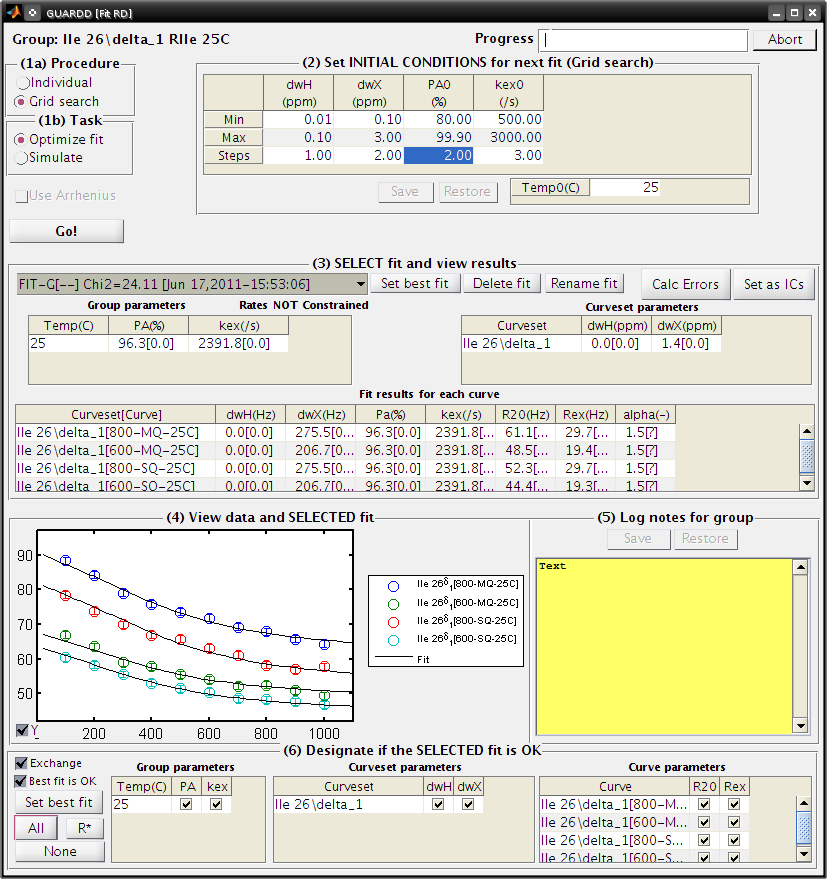
• Note: If unsure about which initial conditions to use, the grid search fits multiple times with different initial conditions
• (1a) Procedure: Grid search
• In the interest of time, use this relatively small grid

dwH(ppm)	dwX(ppm)	PA0(%)	kex0(/s)
Min	0.01	0.1	80
Max	0.1	3.00	99.9
Steps	1	2	2

• Click Save
• (1b): Task: Optimize fit
• Click Go! (5-10 sec/fit x 12 fits = 60-120 sec)
  • Note: Progress can also be viewed in the MATLAB Command Window
• (3) SELECT fit and view results
  • The Fit-G result listed is the best fit (lowest χ²) out of all the 12 fits in the grid search
  • The remaining 11 fits can be viewed in the Chi2 Map window. See the Manual for directions on the χ² Map.
• (6) Designate which parameters are OK
  • Click All

Observe: Becuase the initial conditions used for Fit-1 above were appropriate, both Fit-1 and Fig-G yield the same result

• Note: The grid search can demonstrate success if the optimal fit is insensitive to inital conditions

• Note: Saving data and output plots are discussed later in this document.

Save GUARDD session to file

• In the Main GUARDD window, select the Output tab. Click Save Session As
• GUARDD will create an output folder named with the date, and suggest a filename for you
• Note: To change the default output folder, use the Settings window.

Tip: Save your work often (in case GUARDD and/or MATLAB crashes)

Fit multi-temperature group manually

Use Fit RD window to manually fit one group acquired at multiple temperatures

• Determine optimal P_A and k_ex at each temperature (x3) via two methods (A and B) → propagate to all curves in group
• Determine optimal Δω_H and Δω_X for each curveset (x1) → propagated to all curves in curveset
• Determine and R₂⁰ for each curve (x10)

Demonstrate multi-temperature fitting options

• Method A (No rate constraint): Determine optimal P_A and k_ex at each temperature
• Method B (Impose rate constraint): Determine optimal P_A and k_ex at some temperature T₀ with ΔH and E_AB to determine P_A and k_ex at an arbitrary temperature
• Details: Read more about assigning fitting parameters in the Manual.

Fit without rate constraints (Method A)

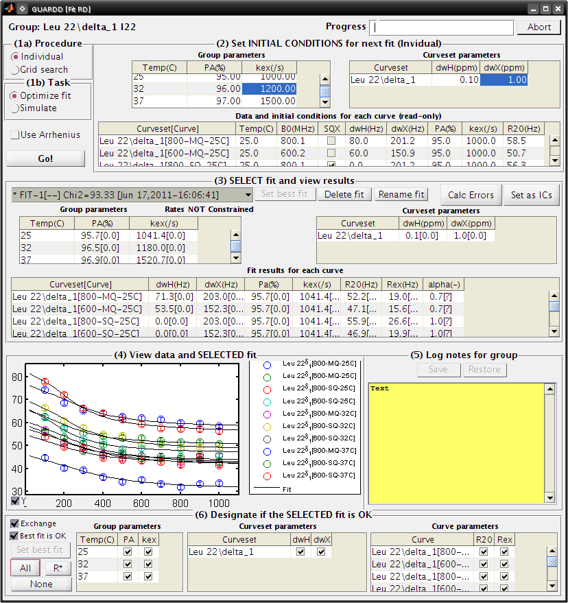
Main GUARDD window - Select Leu 22delta1 - The Fit RD window should automatically open (no double-click required) - If it does not open, check Fit dispersion then select Leu 22delta1

Fit RD Window - (1a) Procedure: Individual - (1b) Task: Simulate - Uncheck Use Arrhenius - Individual initial conditions

Temp(C)	PA(%)	kex(/s)
25	95	1000
32	96	1200
37	97	1500

Curveset	dwH(ppm)	dwX(ppm)
Leu 22delta1	0.1	1

Click Go! (1-5 sec)

• Note that these initial conditions are reasonable (fit is somewhat close to data)
• (1b) Task: Optimize fit
• Click Go! (5-30 sec)
• (3) Select Fit-1[–] fit result
• Click Set best fit
• (6) Designate that all parameters are OK
• Check Best fit is OK
• Click All

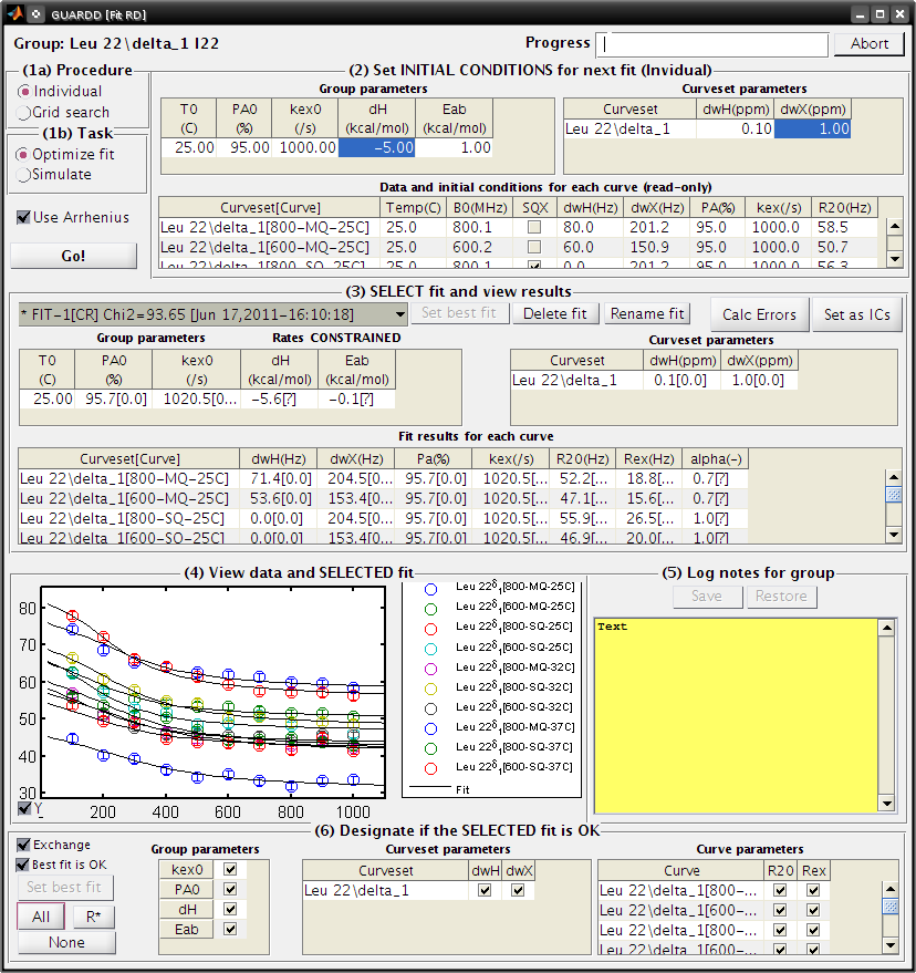
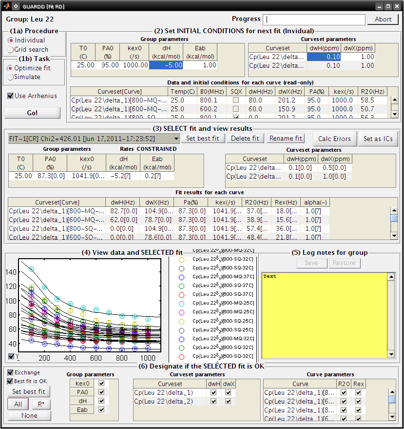
Fit with rate constraints (Method B)

Fit RD

• (1a) Procedure: Individual
• (1b) Task: Simulate
• Check Use Arrhenius
• (2) Individual initial conditions

T0(C)	PA0(%)	kex0(/s)	dH(kcal/mol)	Eab(kcal/mol)
25	95	1000	-5	1

Curveset	dwH(ppm)	dwX(ppm)
L22delta1	0.1	1

Click Go! (1-5 sec)

• Note that these initial conditions are reasonable (fit is somewhat close to data)
• (1b) Task: Optimize fit
• Click Go! (5-30 sec)
• (3) Select Fit-1[CR] fit result
• Click Set best fit
• (6) Designate that all parameters are OK
• Check Best fit is OK
• Click All

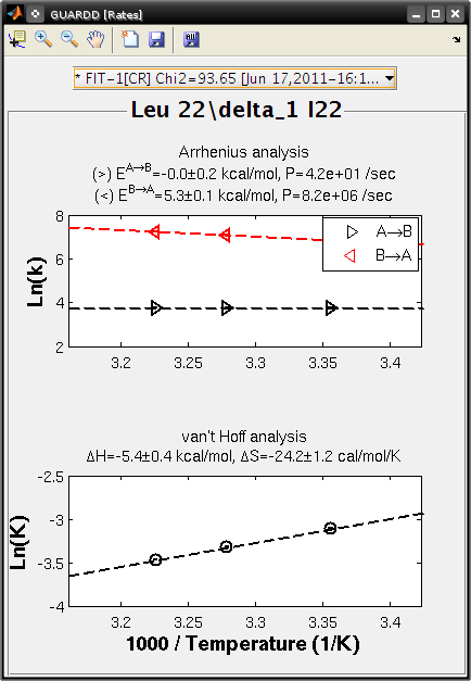
Examine rate analysis (vant Hoff and Arrhenius)

Use Rates window to examine temperature-dependence of rates (vant Hoff and Arrenius)

Main

• Make sure Leu 22delta1 is selected
• Select the Output tab and select Display Rates
• Select fit: Fit-1[–]
• The rates in this fit are independently determined for each temperature
• ΔH, E_AB and E_BA are extracted from the slopes
• Select fit: Fit-1[CR]
• The rates are constrained to lie along the line with slope ΔH, E_AB or E_BA
• Save the figure to a file
• Close Rates

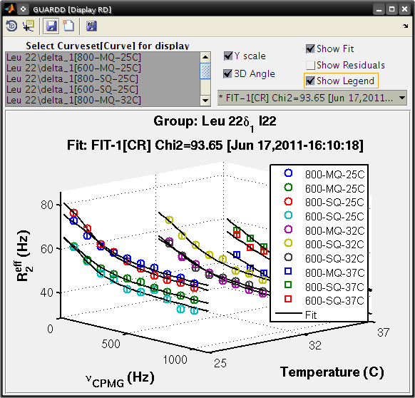
View fits to RD data

Goals

• Use Display RD window to assess the fit to the RD data, and prepare an output figure
• Create a 3D plot that highlights the amount of data in the set

Main

• Make sure Leu 22delta1 is selected
• Output…Display RD…

Display RD

• Select all the curves in the Curveset(Curve) list
• Select fit Fit-1[CR] from fit list
• Check Y scale to auto-scale the Y-axis for this group only
• Check 3D Angle
• Uncheck Show Residuals
• Click Save Figure to Disk icon in taskbar
• GUARDD will prepare a filename for saving, and you must type the file extension
• Type ps to save as a postscript file and click Save (or hit Enter)

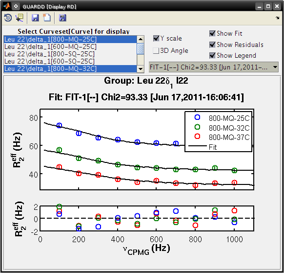
Create a 2D plot with residuals that highlights the fit to some of the data

Display RD

• Select only the following curves from the list

• Curve 1: 800-MQ-25C
• Curve 5: 800-MQ-32C
• Curve 8: 800-MQ-37C

• Select fit Fit-1[–] from fit list
• Uncheck 3D Angle
• Check Show Residuals
• Click Save Figure to Disk icon in taskbar
• GUARDD will prepare a new filename becuase it is a different fit number
• Type ps to save as a postscript file and click Save (or hit Enter)
• Close the Display RD window

Save the session often!

• Main
• Output…Save session as…

Create and fit a multi-curveset, multi-temperature group manually

Prepare and fit a relatively large group of data

Create a multi-curveset, multi-temperature group

Use Data Manager to create a group with multiple curvesets

Main

• Input…Data manager…

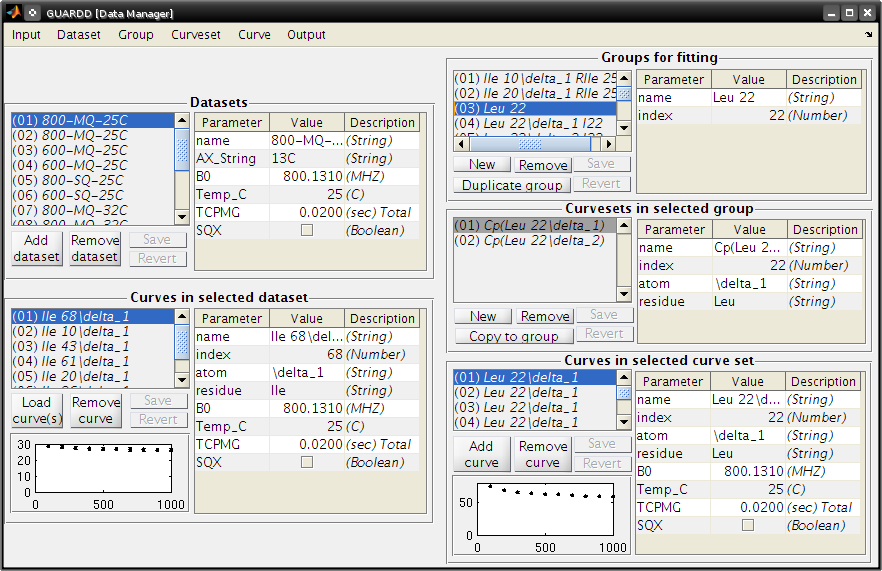
Data Manager

Create a new group for Leu 22

• Click New in the panel Groups for fitting
• Table on right, enter group name: Leu 22
• Table on right, enter group index: 22
• Click Save in the panel Groups for fitting

Add two curvesets to this new group

• Select group Leu 22delta1
• Select curveset Leu 22delta1
• Click Copy to group

Select Group

• Select group Leu 22 (at the bottom)
• Click Select
• Repeat this process with the second curveset, Leu 22delta2

Group -> Sort groups

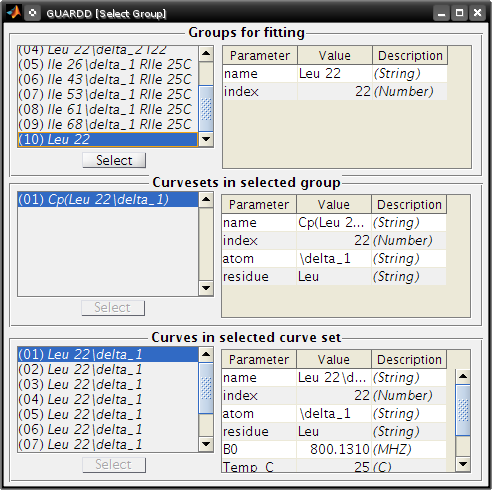
• Make sure that groupLeu 22contains two curvesets: Cp(Leu 22delta1)and Cp(Leu22delta2)
• Note: A copy (“Cp”) is made because this is a different curveset than the original, and therefore may contain a different set of curves (e.g., only one temperature, only MQ)
• It can be renamed if desired, with no adverse effects
• See the manual for more on organizing data
• Close Data Manager

Fit a multi-curveset, multi-temperature group

Use Fit RD window to manually fit one group containing multiple curvesets

Determine optimal P_A and k_ex at each temperature (x3) → propagate to all curves in group

Determine optimal Δω_H Δω_X for each curveset (x2) → propagated to all curves in curveset

Determine and R₂⁰ for each curve (x20)

Main

• Uncheck Fit dispersion so the window does not open automatically
• Click Refresh so the new group appears
• Select Leu 22
• Check Exch?
• Analysis…Fit dispersion…

Fit RD

• (1a) Procedure: Individual
• (1b) Task: Optimize fit
• Uncheck Use Arrhenius
• (2) Individual initial conditions

Temp(C)	PA(%)	kex(/s)
25	95	1000
32	96	1200
37	97	1500

Curveset	dwH(ppm)	dwX(ppm)
Cp(L22delta1)	0.1	1

• Click Go! (50-100 sec)
• (3) Select Fit-1[–] fit result
• Click Set best fit
• (6) Designate that all parameters are OK
• Check Best fit is OK
• Click All

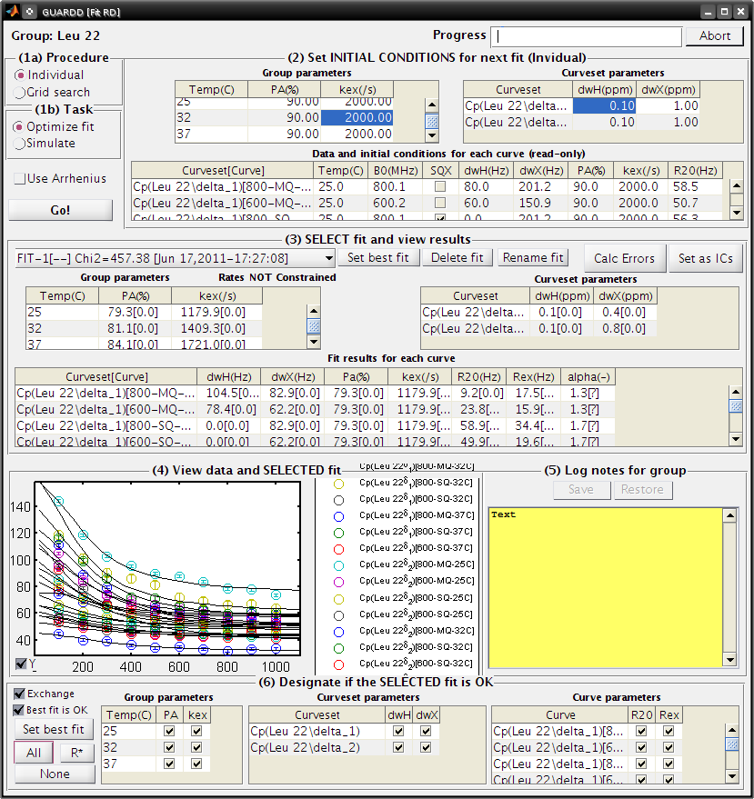
Demonstrate issue that some optimized fits are sensitive to initial conditions (especially noisy and/or many data)

Fit RD

• Fit without rate constraints
• (1a) Procedure: Individual
• (1b) Task: Optimize fit
• Uncheck Use Arrhenius
• (2) Individual initial conditions

Temp(C)	PA(%)	kex(/s)
25	90	2000
32	90	2000
37	90	2000

Curveset	dwH(ppm)	dwX(ppm)
Cp(L22delta1)	0.1	1

Click Go! (50-100 sec)

(3) Select Fit-1[–] fit result

(6) Designate that all parameters are OK

• Check Best fit is OK
• Click All

Observe: This optimized fit is significantly different than previous Fit-1[–]

Fit	PA(%)	kex	Chi2
First	87.4	1094.0	394.78
Second	79.3	1179.9	457.38

• There are systematic ways to assess quality of fit. These methods are covered later in this tutorial
• Close Fit RD window

Save the session often

Main

• Output…Save session as…

Perform batch task

Fit several groups sequentially to obviate need for user input

Main

• Analysis…Batch task…

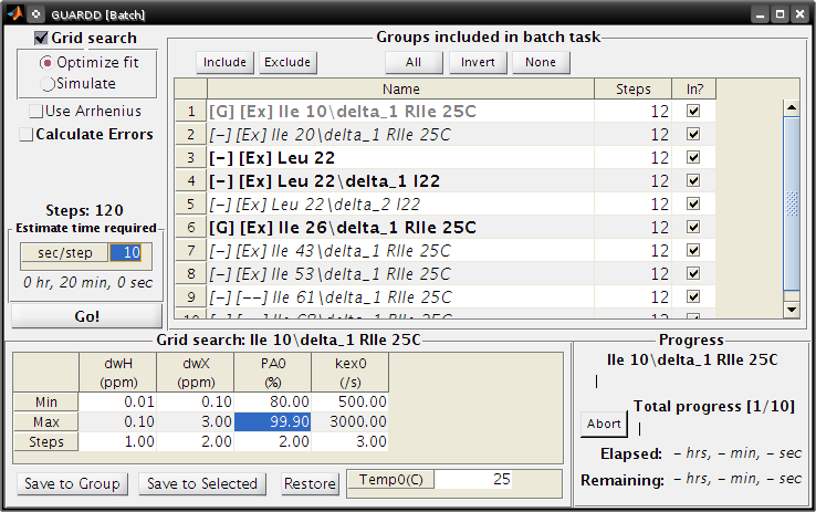
Batch

• Select groups for analysis
• Highlight rows corresponding to each group
• Click Include button
• Note: The checkboxes are read-only (not clickable, sorry!)
• Specify the task
  • Grid search: Optimize fit
  • Use Arrhenius: Unchecked
  • Note: Fixing Arrhenius analysis adds two more dimensions to the grid search (dH and Eab)
  • Errors: Unchecked
  • Click on any one row to specify grid search limits

	dwH(ppm)	dwX(ppm)	PA0(%)	kex0(/s)
Min	0.01	0.1	80	500
Max	0.1	3.00	99.9	3000
Steps	1	2	2	3

• Note: The tutorial file included in GUARDD v.2011.09.11 session uses Steps = 2, 3, 5, 5 for a total of 150 points, instead of Steps = 1, 2, 2, 3 (60 points) shown here in v.2011.07.01

Click Save to Selected to save thid grid to all of the groups in the batch

Estimate time required

• This calculator will help plan the time required for an estimated steptime
• As seen in the tutorial, each fit step may take 5-100 sec, depending on the size of data and accuracy of initial conditions
• Estimate 10 sec/step, for a total of ~20 min
• Click Go!

Note: After each group step is done, a session file “GUARDD-Session–Batch_Progress.mat: is written to the default output directory

This was designed for two purposes

• In case the program crashes, progress is saved
• Allows the user to start a batch task on one computer (e.g., at work), then download/view the results remotely on another computer (e.g., at home)

Time for a break?

• This is a good stopping point in the tutorial, in case you want to resume later
• The batch task does not need to be completed
• The tutorial proceeds using a pre-saved GUARDD session

Assess quality of fit

Determine how well RD parameters are determined and which parameters are OK

• Increasingly challenging for larger and/or noisier datasets

Methods of assessment

Check fit to data and the resulting residuals

• A well-determined fit yields residuals randomly distributed about zero (i.e., not systematically shaped)

Check sensitivity of fit to initial conditions (grid search)

• A well-determined fit is insensitive to initial conditions

Check sensitivity of fit to errors in data (Monte Carlo errors)

• A well-determined fit yields a narrow set of MC-fits from Monte Carlo analysis

Check exchange-timescale parameter α

• Fast exchange (k_ex>>Δω; α→2.0) precludes knowledge of P_A and Δω
• This is often evident in prior steps

Load GUARDD session with data already fit

Main

• Input…Load session…
• Select tutorial file:

tutorial/data/GUARDD-Session-Tutorial.mat

or

GUARDD-Session--Tutorial-After_Break.mat}}}

in v.2011.09.11

• This session contains data from above, with completed 60-point grid search and MC errors
• Focus on two examples

Leu 22delta1, a good fit with known parameters

• Medium dataset (10 curves)
• α = 1.0: intermediate exchange
• Grid search: fit is sensitive to ICs, but well-defined solution at min(χ²)
• MC Errors: model example, symmetric about optimum solution
• Parameters: All are known

Ile 43, a good fit with unknown parameters

• Small dataset (4 curves)
• α = 1.4-1.9: fast exchange
• Grid search: two solution with different values
• MC Errors: very wide, reflecting many fitting soltuions
• Parameters: P_A and Δω unknown

View fit and residuals

Goal: View the RD fit and residuals to help assess fit quality

• Confer prior tutorial steps on using the Display RD window

View Grid Search Chi2 Map for good fit

Goal: Assess the extent to which fitting is sensitive to initial conditions

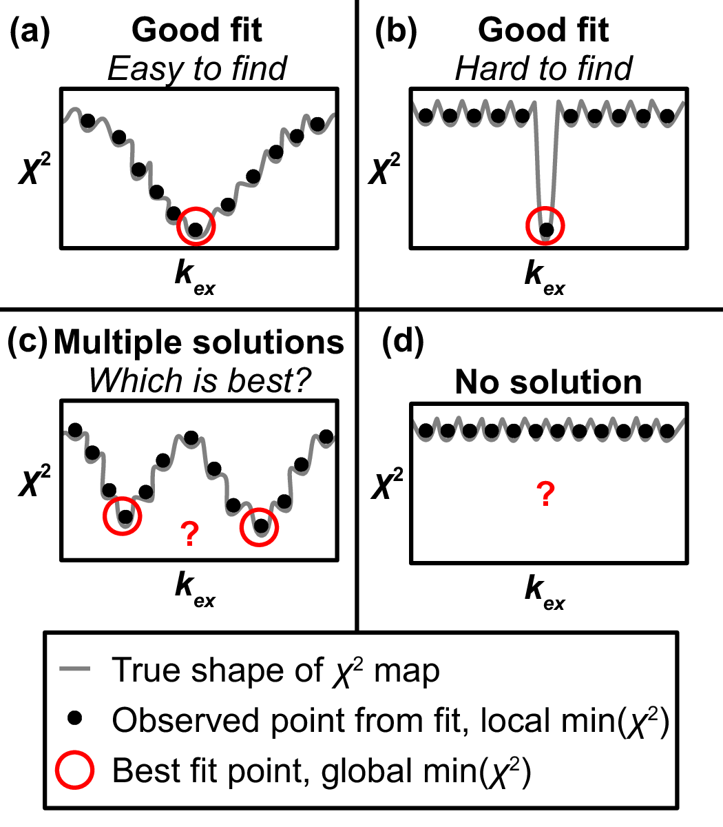
Key info on features of chi2 maps

• A Chi2 map displays a set of parameter values (e.g., for k_ex) on the X-axis and the goodness of fit (χ²) associated with that value on the Y-axis
• The most precise fit is at the min(χ²)
• Chi2 maps take a variety of shapes, such as “.”, “U”, “W”, and “-“
• *Details*: Read more in the Manual

Goal: Use both Chi2 Map window and Fit RD window to view data

Main

• Select Leu 22delta1
• Output…Display chi2 map…
• Analysis…Fit dispersion…

Chi2 Map

• Parameters: dwH, dwX, Pa, kex
• Curveset (Curve): 800-MQ-25C, 800-MQ-32C, 800-MQ-37C
• Top% slider all the way to the top (100%)
• Fit: FIT-G[–] Chi2=93.33
• Task to Display: Grid Search
• Results to Display: Final
• Display Mode: Scatter

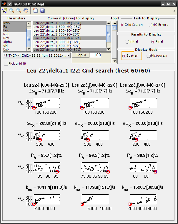
Goal: Interpret the Grid Search results the Chi2 Map window

Each subplot shows a single parameter on the X-axis, and its different values in different fits

Each black point corresponds to ONE optimized fit result

There are 60 fits in this example (hence 60 points in each subplot), each of which started from a different location in parameter space (note tutorial file in GUARDD v.2011.09.11 uses 150 points instead of 60)

Those initial locations can be displayed by setting Results to display: Initial

The red circle designates the currently selected fit result

The blue square designates the best fit from the grid search

Clicking Pick grid fit will allow selection of any of the grid fits shown

• The green diamond designates the currently selected fit from the displayed grid list
• Any of these can be added to the list of fits, if desired

Observe: The fit to the no exchange model is inappropriate

Chi2 Map

1. Select Fit: NoEx[–]
2. The χ² = 2163.58, which is very large
3. The 60 optimized fits are well below this value

Fit RD

1. Select Fit: NoEx[–]
2. The fit is a poor representation of the data

Observe: The best fit is appropriate since the chi2 map remain U-shaped near the best result

Chi2 Map

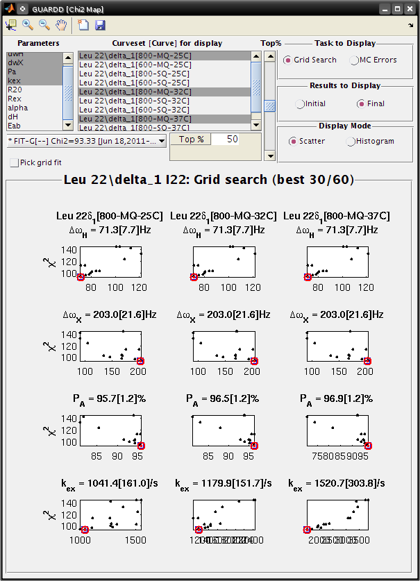
1. Select Fit: FIT-G[–] Chi2=93.33
2. Move the Top% slider down to 50% in 4-6 small steps
3. Observe: The chi2 map remains U-shaped even as the poorest fits are eliminated from display

View Monte Carlo Errors χ² Map for good fit

Goal: Assess the extent to which fitting is sensitive to noise in the data

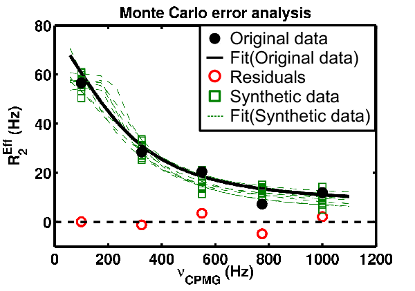
Key info on Monte Carlo analysis

• The goal of MC analysis is to generate and fit many synthetic datasets which differ from one another by an amount related to the goodness of fit to the original data
• Each synthetic dataset will have a different set of optimal fit values (e.g., P_A k_ex)
• The distribution of fitted values reflects the degree to which the original data define its own optimal values
• Example: A worse optimal fit to the original data yields more different MC datasets and therefore more differentoptimal parameter values
• Details: Read more about Monte Carlo error estimation in the Manual

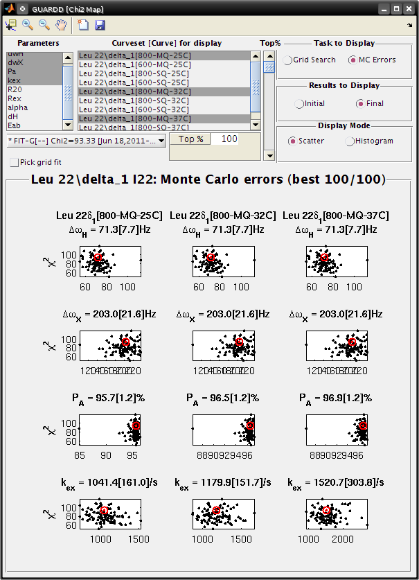
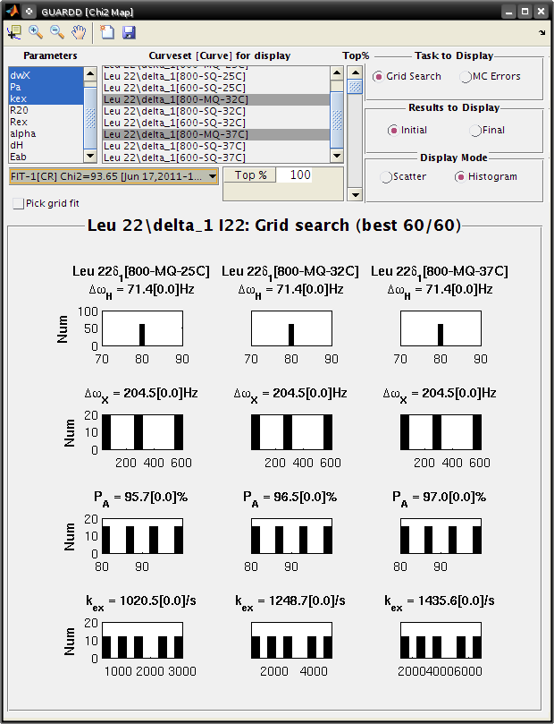
Chi2 Map

1. Make sure Fit: FIT-G[–] Chi2=93.33 is selected
2. Set Top% slider all the way to the top (100%)
3. Task to Display: MC Errors
4. Results to Display: Final
5. Display Mode: Scatter

Goal: Interpret the MC Errors results in the χ2 Map window

Each subplot shows a single parameter on the X-axis, and its different values in different fits

Each black point corresponds to ONE optimized fit result to a synthetic MC dataset

• There are 100 fits in this example (hence 100 points in each subplot), each of which corresponds to a synthetic MC dataset
• The initial conditions to each fit are given by the best fit to the original data (see Results to display: Initial)

The red circle designates the best fit to the original data

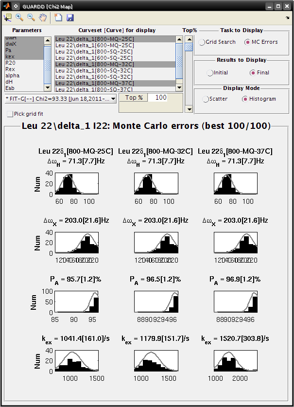
Set Display Mode: Histogram

The gray lines show the hypothetical distributions reflecting “errors” in the data

• The mean of each distribution is from the best fit value to the original data
• The standard deviation of each distribution is the standard deviation from the distribution of MC fitted values
• Each deviation is reported as the “error” in each fitted parameter (shown in brackets)
• Note: it is usually best to use a Top% =100% for MC errors
• Sometimes anomalous fits yield very large χ², and can be discarded, but this is rare

Observe: The symmetry of the MC χ² maps indicate reliable estimation of error, and is consistent with reasonable parameter values

• The scatter plot illustrates a circular distribution about the optimal result
• The histogram is roughly symmetric, and is well-described by the standard deviation

View Grid Search χ² Map for fit with unknown parameters

Goal: Illustrate features of Grid Search and MC Errors which correspond to a partially-defined fit

Ile 43, a good fit with unknown parameters

• Small dataset (4 curves)
• α = 1.4-1.9: fast exchange
• Grid search: two solution with different values
• MC Errors: very wide, reflecting many fitting soltuions
• Parameters: P_A and Δω unknown

Main

1. Select Ile 43 delta1
2. Output…Display chi2 map…
3. Analysis…Fit dispersion…

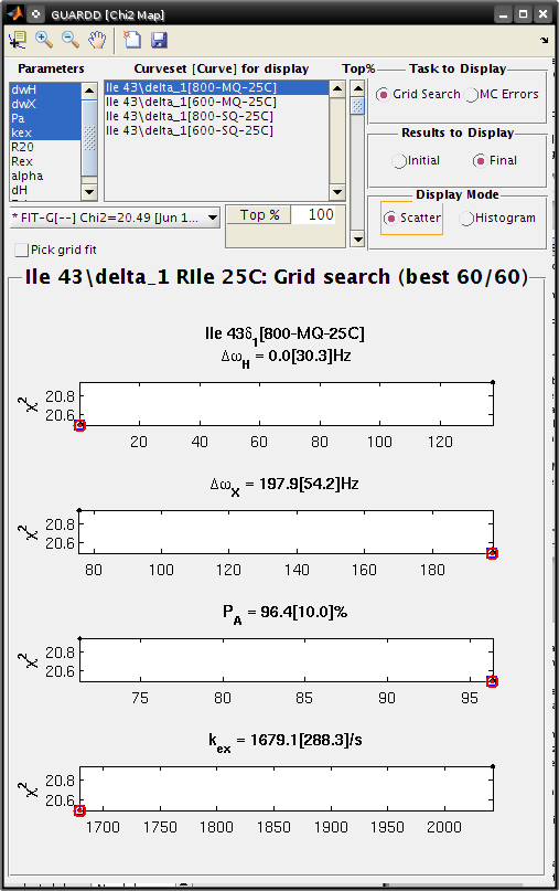
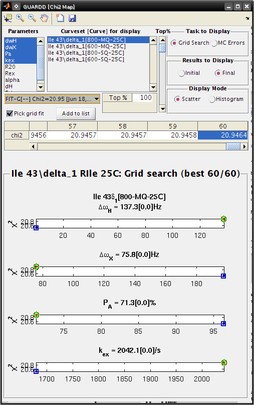
Chi2 Map

1. Parameters: dwH, dwX, Pa, kex
2. Curveset (Curve)*: 800-MQ-25C
3. Top% slider all the way to the top (100%)
4. Fit: FIT-G[–] Chi2=20.49
5. Task to Display: Grid Search
6. Results to Display: Final
7. Display Mode: Scatter

Observe: The grid search illutrates solutions at two distinct points

Goal: Add the higher-χ² fit to the fit list for further inspection

Chi2 Map

1. Check Pick grid fit
2. Scroll to the right, and select fit number 60, chi2=20.9464 (or number 93, 20.9456 in v.2011/09/11)
3. The green diamond should highlight this fit
4. Click Add to list
5. The fit FIT-G[–] Chi2=20.95 is now highlighted by the green diamond and red circle (since it is selected)

Fit RD

1. (3) SELECT the new fit FIT-G[–] Chi2=20.95 from the list
2. Note: if it is not shown, the list can be update by re-selecting any fit on the list (then check again)
3. Observe: These two fits both appear to go through the data! (which one is best?)
4. Note: Residuals can be compared using the Display RD window

For now, we will continue to analyze the lower-χ² fit

View Monte Carlo Errors χ² Map for fit with uknown parameters

Goal: Illustrate features of Grid Search and MC Errors which correspond to a partially-defined fit

Chi2 Map

1. Make sure Fit: FIT-G[–] Chi2=20.49 is selected
2. Set Top% slider all the way to the top (100%)
3. Task to Display: MC Errors
4. Results to Display: Final
5. Display Mode: Scatter
6. Observe: A wide range of Δω and P_A values can describe these data → Δω and P_A are not OK!
7. Close Chi2 Map window

Goal: Mark these parameters as “Not OK” in the Fit RD window

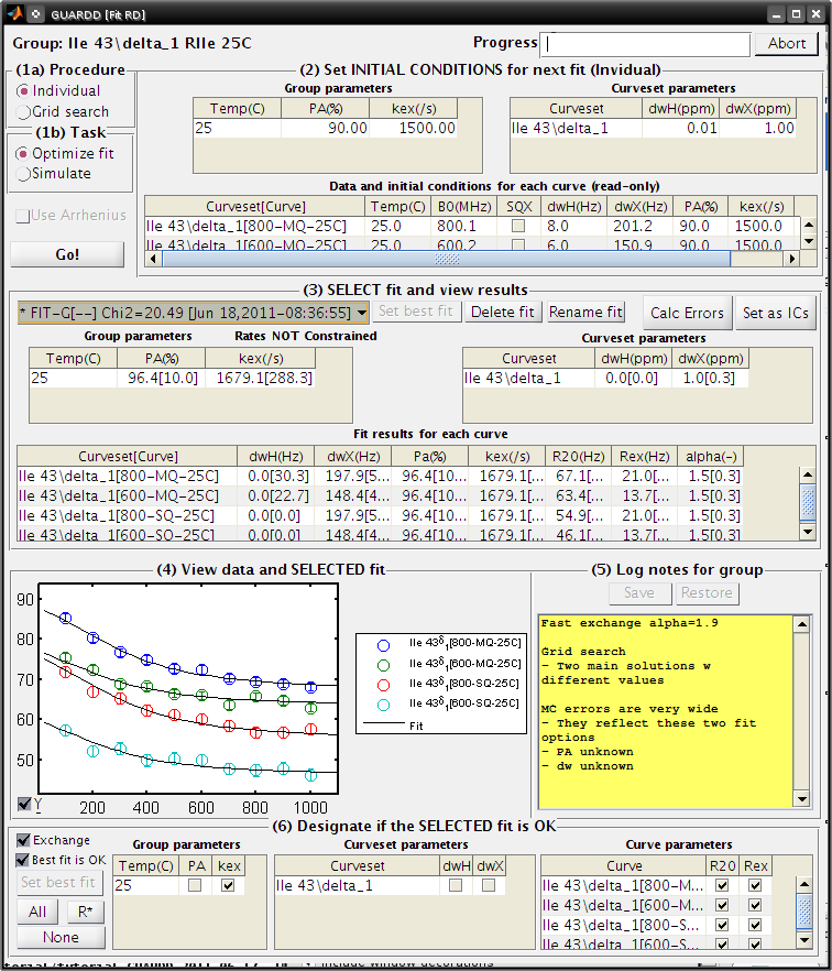
Fit RD

1. (3) SELECT the fit FIT-G[–] Chi2=20.49 from the list
2. (6) Designate which elements of this fit are OK
3. Exchange: check
4. Best fit is OK: check
5. Click Set best fit, if possible (should be “best” already)
6. Cilck All
7. Group parameters: uncheck P_A
8. Curveset parameters: uncheck both dwH and dwX
9. Make note of this in the (5) Log notes for group panel (or take note of the current note)
10. Close Fit RD window

Document notes for organization

Goal: View and maintain organized notes for interpreting fit results

Main

1. Analysis…Notes…

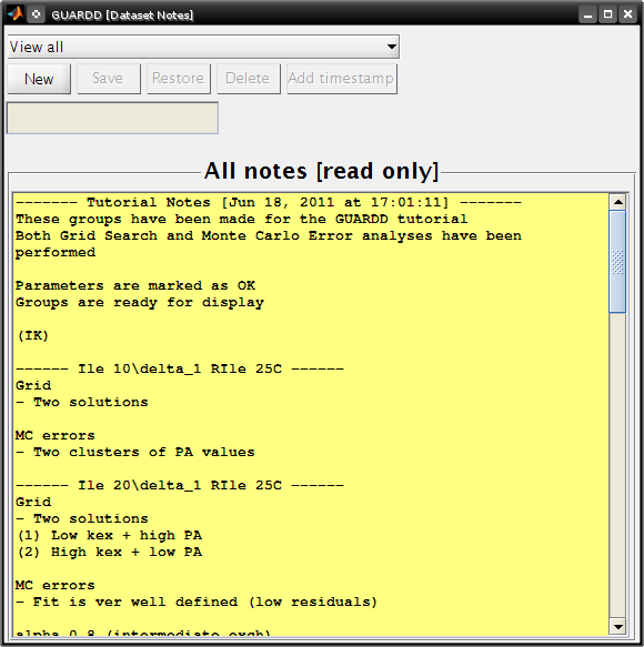
Notes

1. Notes on groups are edited in the Fit RD window
2. Notes on the session can be created and edited in the Notes window
3. Close the Notes window

Output results

Goal: Aggregate and output any/all results for dissemination

View results in display cluster

Goal: Visual display of results from all groups

Goal: Load GUARDD session with data already fit (in case this has not been done already)

Main

1. Input…Load session…
2. Select tutorial file:

tutorial/data/GUARDD-Session-Tutorial.mat

or

GUARDD-Session--Tutorial-After_Break.mat

in v.2011.09.11

This session contains data from above, with completed 60-point grid search and MC errors (150 point grid for tutorial file in GUARDD v.2011.09.11)

Goal: Create two display groups to compare different fitting constraints

Main

• Output…Display group results…

Groups

1. Click New
2. Set name: Isolated fits
3. Click Save
4. Panel All Groups, select all groups except Leu 22
5. Click Add
6. Click New
7. Set name: Group fits
8. Set RGB to 1 0 0 (for the color Red)
9. Click Save
10. Panel All Groups, select only Leu 22
11. Click Add

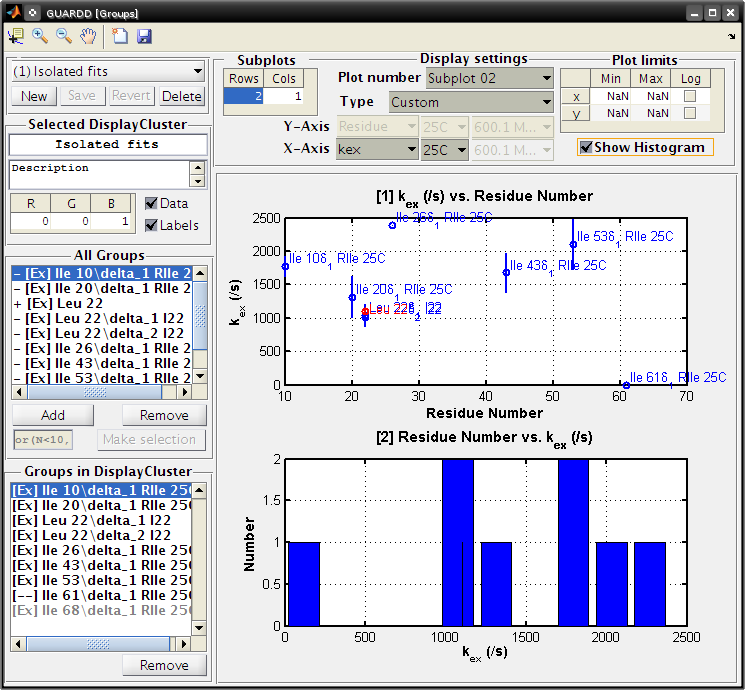
Goal: Compare individual fits from each NMR probe to form candidate groups, identify outliers, etc.

Groups

Panel

Display settings

Select plot type: Kinetic rate (25C)

Note: Differences in k_A and k_B values indicates the extent of site-specific motion in the protein

Note: Global fit for Leu 22 (red) is close to both individual fits for Leu 22δ_1 and Leu 22δ_2 (blue)

Set Subplots: Rows=2, Cols=1

Plot number: Subplot 01

• Type: Custom
• Y-Axis: kex, 25C
• X-Axis: Residue

Plot number: Subplot 02

• Type: Custom
• Check Show Histogram
• X-Axis: kex, 25C

Click the Save Figure icon in the title bar

• GUARDD will prepare a filename for saving, and you must type the file extension
• Type ps to save as a postscript file and click Save (or hit Enter)

Close Groups window

Bug: Selecting dwX_ppm results in an error involving iscolumn() in some versions of MATLAB (at least R2009a on Windows)

View results in table

Goal: Aggregate and output any/all results for dissemination

1. Main
2. Output…Display results table…
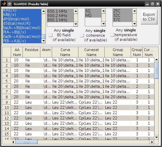
3. Results Table
4. Select all display parameters in left-most list
5. Select all conditions in the following three lists
6. Click Export to CSV

Bug: Selecting all items in the table results in an error in some versions of MATLAB (at least R2009a on Windows)

Export data and groups

Goal: Aggregate and output results for dissemination

Main

• Input…Data manager…

Data Manager

1. Output…Datasets…
2. Save the file

• This copies all imported datasets
• Output…Groups…

1. Save the file
2. Contains all groups, curvesets, and curves created for analysis

Simulate and export RD data

Goal: Explore the nature of RD phenomena

• Question: What are limits of detection (i.e., when is R_ex>0)?

Simulate multi-field dataset

Goal: Simulate a simple dataset at two magnetic fields

Main

• Input…RD Simulator…

RD Simulator

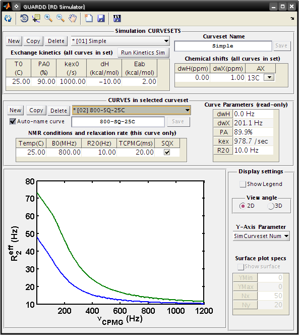
Create a new SimCurveset, which specifies kinetics and chemical shifts for all curves within

1. CURVESETS: Click New
2. Set Name to Simple
3. Click Save

Create a new SimCurve, which specifies NMR conditions for simulation

1. CURVES: Click New
2. Set B0(MHz) to 500
3. CURVES: Click New

Simulate multi-field, multi-temperature dataset

Goal: Simulate a dataset at two magnetic fields and three temperatures

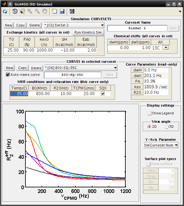
RD Simulator

Create a new SimCurveset

1. CURVESETS: Click New

Create two new SimCurves at 15C (500 MHz and 800 MHz)

1. CURVES: Click New
2. Set Temp(C) to 15
3. Set B0(MHz) to 500
4. CURVES: Click New
5. Set Temp(C) to 15

Create two new SimCurves at 25C (500 MHz and 800 MHz)

1. CURVES: Click New
2. Set B0(MHz) to 500
3. CURVES: Click New

Create two new SimCurves at 35C (500 MHz and 800 MHz)

1. CURVES: Click New
2. Set Temp(C) to 35
3. Set B0(MHz) to 500
4. CURVES: Click New
5. Set Temp(C) to 35

Explore experimental condtions for observing RD

Goal: Explore the nature of RD phenomena using surface plot

Note: Please complete prior tutorial section before proceeding

Question: What temperature range is appropriate for acquisition?

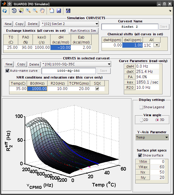
RD Simulator

1. Display settings: click 3D angle
2. Set Y-Axis Parameter to Temp
3. Check Show surface

Observations

1. For these exchange kinetics, the largest dispersions are observed around 10-20C, and therefore experiments should be focused there
2. The RD curve is nearly undetectable above 50C because k_ex is too large compared to Δω_X(Hz)

Change chemical shift to observe the effect on the RD signal

CURVESET: Set *dwX(ppm)* to 0.50

Observations

1. With smaller Δω_X(ppm), the dispersions are smaller, because k_ex is larger in comparison

CURVESET: Set *dwX(ppm)* back to 1.00

Change magnetic field strength to observe the effect on the RD signal

CURVE: Set B0(MHz) to 1000

Observations

1. At higher field strength, dispersions are larger, becuse Δω_X(Hz) is increased

Explore temperature-dependence of exchange kinetics

Goal: Explore the nature of exchange kinetics using the Kinetic Simulator

Note: Please complete prior tutorial section before proceeding

RD Simulator

1. Start the Kinetic Simulator
2. CURVESET: Click *Run Kinetics Sim*

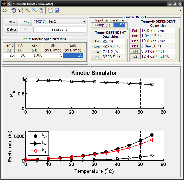
Kinetic Simulator

• This window operates on the Sim Curvesets, and displays the effect of temperature on the RD parameters P_A and k_ex

1. Select SimSet 2 from the pull-down menus
2. Alter the kinetic parameters in the Input Kinetic Specifications table
3. Set dH to 5
4. Now, P_A will decrease with increasing temperature
5. Set Eab to 15
6. This ensures that k_ex still increases with temperature
7. Check the Kinetic Report for the quantitative values of exchange parameters
8. Set Input temperature to 50

Observe: P_A is 82.4% and k_ex is 4039.7 /s

Check this effect on the simulated RD surface plot

RD Simulator

1. Click the Refresh display icon in the title bar
2. Observe: The RD signal now increases with temperature, because the population of the minor state, P_B = (1-P_A), becomes larger at higher temperatures

Kinetic Simulator

• Close the window (X)

Export simulated data

Goal: Assess accuracy of fitting procedure by analyzing data with “known” solution

Note: Please complete prior tutorial section before proceeding

RD Simulator

1. Click the Export icon in the title bar

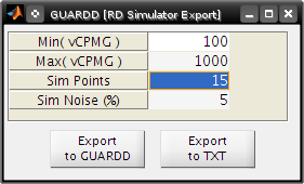
RD Simulator Export

1. Set Sim Points to 15
2. Click Export to TXT
3. Save the file

RD Simulator

1. Click the Export icon in the title bar
2. Set Sim Points to 15
3. Click Export to GUARDD

• This automatically creates a Group for each simulated Curveset
• Note 3: Simulated groups can be viewed in the Main window and/or the Data Manager, just like any other group
• Fitting can be accomplished as per the simple group or for the multi-temperature group.
• Fits of these data should achieve within 10% accuracy of the simulation conditions

This concludes the tutorial!